2. Mathematical Foundations
This chapter covers the mathematical foundations for digital circuit design. Most importantly, we introduce binary numbers and Boolean algebra. Furthermore, we discuss methods to determine the extrema of functions for use in the context of minimizing the delay of a circuit, including arithmetic and geometric means, root finding for polynomials, and elementary calculus.
2.1. Numbers
Digital circuits use voltages to encode information including numbers. Among various alternatives, binary numbers have emerged as the best match for digital circuits. Athough the encoding of binary numbers with low and high voltages differs from our familiar decimal number system, the underlying principles are essentially the same. In the following, we discuss the representation and manipulation of numbers in the binary number system.
2.1.1. Positional Number Systems
We are all familiar with numbers as a concise abstraction for counting concrete quantities like two apples or seven oranges. Most of us associate a magnitude with a number like 4362. If you think this number is large, it’s perhaps because you are just wondering about how big a pile of 4362 apples might be. If, on the other hand, you are saving money for a trip into space, then 4362 Euros are too little to get you even close. Deeper thoughts about number 4362 reveal that it is a juxtaposition of the four digits 4, 3, 6, and 2, with an order that matters. Each digit counts a quantity. Digit 2 counts ones, digit 6 counts tens, digit 3 counts hundreds, and digit 4 counts thousands. The value of the number 4362 is actually the sum of the counts:
\(4362\ =\ 4 \cdot 1000 + 3 \cdot 100 + 6 \cdot 10 + 2 \cdot 1\,.\)
Here is another number with the same value 4362:
These Babylonian cuneiform symbols may look unfamiliar, but
the underlying rules to determine the value of the number are
identical. The symbols count quantities. Symbol  denotes
1, symbol
denotes
1, symbol  denotes 12, and
  denotes 42. Given
the order of the three symbols, the rightmost symbol counts
ones, symbol counts sixties, and symbol counts
threethousandsixhundreds. The value of the number is the sum of the
counts:
denotes 42. Given
the order of the three symbols, the rightmost symbol counts
ones, symbol counts sixties, and symbol counts
threethousandsixhundreds. The value of the number is the sum of the
counts:
\(\ =\ 1 \cdot 3600 + 12 \cdot 60 + 42 \cdot 1\ =\ 4362\,.\)
Fourthousand years ago, a Babylonian might have looked at the number,
and would have been in awe about a pile of apples just
like we are about a pile of 4362 apples today.
We do not suggest that digital circuits are capable of imagining how big a pile of
\(1\,0001\,0000\,1010\)
apples might be. But, this number has value 4362 as well, and the value can be derived by the same counting rules. Each digit 0 or 1 counts quantities that are powers of 2:
\[\begin{eqnarray*} 1\,0001\,0000\,1010 &=& 1 \cdot 4096 + 0 \cdot 2048 + 0 \cdot 1024 + 0 \cdot 512 + 1 \cdot 256 + 0 \cdot 128 + 0 \cdot 64 + 0 \cdot 32 + 0 \cdot 16 + 1 \cdot 8 + 0 \cdot 4 + 1 \cdot 2 + 0 \cdot 1 \\ &=& 4362\,. \end{eqnarray*}\]
The three numbers above represent value 4362 in three different forms with a common set of rules known as positional number system. The Babylonians were among the first to use a positional number system.[1] They were concerned about recording their number symbols with a stylus on clay tablets. Our familiar ten digits \(0, 1, 2, \ldots, 9\) seem to have their origins in counting with ten fingers or perhaps toes. In contrast, bits 0 and 1 are abstract representations of low and high voltages in digital circuits.
In a positional number system, number \(N\) is a juxtaposition of digits, optionally with a radix point to separate the integral and fractional parts:
Number \(N\) has an integral part of \(q\) digits \(a_i\) in position \(i,\) where \(0 \le i < q,\) and a fractional part of \(p\) digits with position \(i\) in range \(-p \le i < 0.\) The number system has an implicit base \(b.\) Digit \(a_i\) in position \(i\) is in range \(0 \le a_i < b.\) A number system with base \(b\) has \(b\) digits. Leftmost digit \(a_{q-1}\) is the most significant digit of number \(N,\) and rightmost digit \(a_{-p}\) is the least significant digit. The least significant digit of integral numbers is \(a_0,\) because they do not have a fractional part. The value of number \(N\) is the value of the polynomial:
The positional notation is a convenient shorthand for this polynomial where the digits are the counts of the powers of base \(b.\) We say that \(b^i\) is the weight of digit \(a_i.\) Our familiar decimal number system has base \(b=10\) with ten digits \(0, 1, \ldots, 9.\) Therefore, the value of integer number 4362 is
\(4362 = 4 \cdot 10^3 + 3 \cdot 10^2 + 6 \cdot 10^1 + 2 \cdot 10^0\,.\)
Analgously, the Babylonian number system is sexagesimal with base
\(b=60.\) Thus, the Babylonians needed sixty digits. They did
not invent sixty different hieroglyphs, but used just two different
cuneiform shapes, the wedge and the chevron  , to
compose the digits. By associating the chevron with value 10, we find
that symbol denotes value 12, because one chevron and two
wedges have value \(10 + 1 + 1 = 12.\) Similarly, has
four chevrons and two wedges with value \(4 \cdot 10 + 1 + 1 =
42.\) In fact, the Babylonians mixed a decimal system for the digits
into the sexagesimal number system, such that
, to
compose the digits. By associating the chevron with value 10, we find
that symbol denotes value 12, because one chevron and two
wedges have value \(10 + 1 + 1 = 12.\) Similarly, has
four chevrons and two wedges with value \(4 \cdot 10 + 1 + 1 =
42.\) In fact, the Babylonians mixed a decimal system for the digits
into the sexagesimal number system, such that
The binary number system with base \(b=2\) has two digits, bits 0 and 1. It is the positional number system with the fewest digits and the longest strings of digits to represent a number, including
\(1\,0001\,0000\,1010\ =\ 1 \cdot 2^{12} + 0 \cdot 2^{11} + 0 \cdot 2^{10} + 0 \cdot 2^9 + 1 \cdot 2^8 + 0 \cdot 2^7 + 0 \cdot 2^6 + 0 \cdot 2^5 + 0 \cdot 2^4 + 1 \cdot 2^3 + 0 \cdot 2^2 + 1 \cdot 2^1 + 0 \cdot 2^0\ =\ 4362\,.\)
When implementing circuits to store and manipulate numbers, a key issue is the number of digits that our circuits can support. More specifically, we may ask how many digits \(q\) we need to represent integral number \(N.\) In a positional number system with base \(b,\) the answer is the smallest \(q\) such that \(N < b^q.\) In terms of the logarithm to base \(b\) [2] and the ceiling function, the smallest number of digits to represent integer \(N\) is
Conversely, we may ask how many integral numbers we can represent with \(q\) digits. In a positional number system with base \(b,\) the answer is \(b^q\) numbers in range \([0, b^q - 1].\) This bracket notation lists the smallest integer 0 and the largest integer \(b^q - 1\) of the range. The examples below illustrate these insights.
Determine the number of digits \(q\) that we need to represent number \(N = 89\) in the decimal and the binary number systems.
By default, we interpret number \(N=89\) as a decimal number with base \(b=10,\) because this is how we were trained to interpret numbers. Since \(N=89\) has two digits, namely 8 and 9, we obviously need \(q=2\) digits to represent \(N\) as a decimal number. We confirm this trivial observation by checking that \(89 < b^q = 10^2 = 100.\) We conclude that we do not need 3 digits to represent 89. On the other hand, if we had 1 digit only, then \(10^1 = 10 < 89\) violates the condition \(N < b^q.\) Therefore, 1 digit is not sufficient to represent 89. Our formula \(q = \lceil \log_b N\rceil = \lceil \log_{10} 89\rceil\) produces the same result \(q = 2\) when evaluated blindly.
If we wish to represent \(N=89\) as a binary number with base \(b=2,\) the formula yields \(q = \lceil \log_2 89\rceil = 7,\) that is we need 7 bits to represent 89 as a binary number. Alternatively, we could have used a trial-and-error strategy to find the smallest power of 2 such that \(N < 2^q.\) Pick \(q = 4,\) and we find that \(q=4\) does not qualify, because \(2^4 = 16\) is not larger than \(N=89.\) Similarly, \(q=6\) yields \(2^6 = 64,\) which is still smaller than 89. The next larger value \(q = 7\) produces \(2^7 = 128,\) which is larger than 89, indeed. Since 7 is the smallest \(q\) such that \(89 < 2^q,\) we need 7 bits to represent 89 as a binary number.
How many integral numbers can we represent with \(q=8\) digits in the decimal and binary number systems?
We know that we can represent \(b^q\) numbers in range \([0,b^q-1]\) in a positional number system with base \(b.\) Thus, \(q=8\) digits in the decimal number system are good for \(10^8\) = 100,000,000 numbers. We can enumerate these numbers as a sorted list:
The smallest number of the list is \(0000\,0000 = 0,\) and the largest is \(9999\,9999 = 10^8 - 1.\) The bracket notation summarizes this range of integers compactly as \([0, 10^8-1].\)
In the binary number system, \(q=8\) digits or bits can represent only \(b^q=2^8=256\) numbers in range \([0,b^q-1]=[0,255].\) The sorted list of 8-bit binary numbers is:
The smaller the base of a number system is, the smaller is the number range that we can represent with a given number of digits \(q.\)
We may invent a new positional number system by choosing a base and symbols for the digits. The hexadecimal number system is a relatively new number system that gained traction in the \(20^{th}\) century when computer technology emerged. The base of the hexadecimal system is \(b=16.\) Thus, we need sixteen digits. Since the 10 decimal digits are not enough, the hexadecimal system borrows the first six letters of the alphabet as symbols for the digits beyond 9:
hexadecimal digit 0 1 2 3 4 5 6 7 8 9 A B C D E F decimal value 0 1 2 3 4 5 6 7 8 9 10 11 12 13 14 15
The value of hexadecimal number CAFE is
and the FBI has value
if we insist on reading letter I as number 1.
We need \(q = \lceil \log_{16} 89\rceil = 2\) hexadecimal digits to represent number 89, just as many as decimal digits. However, the same number of hexadecimal digits enable us to represent many more numbers than in the decimal system. For comparison with Example 2.2, hexadecimal numbers with \(q = 8\) digits can represent \(b^q = 16^8 = 4{,}294{,}967{,}296\) numbers in range \([0,16^8-1].\)
2.1.2. Number Conversion
Number conversion is the process of changing the representation of a number from one number system into another. The value of the number is not affected. For the sake of clarity, we make the system of number \(N\) explict by annotating the base as a subscript, as in \(N_b.\) For example, we interpret \(11_{10}\) as decimal number eleven, and \(1011_2\) as binary number with value eleven. Thus, equality \(11_{10} = 1011_2\) makes sense whereas \(11 = 1011\) does not.
Converting a number from any positional number system into decimal is easy, because we are used to decimal arithmetic. All we need to do is evaluate the polynomial expression of the number. This process is called positional conversion. For example, converting binary number \(1011_2\) into decimal yields:
Converting a decimal number into another system requires a little more work. The conversion algorithm is called successive division, and works as follows: Initially, find the largest power \(p\) of base \(b\) less than or equal to \(N_{10}.\) Then, divide \(N_{10}\) by \(b^p,\) record quotient \(Q = N_{10}/b^q\) as digit \(a_p = 1\) in position \(p,\) and repeat the division with remainder \(R = N_{10} - Q \cdot b^p\) and next smaller position \(p-1\) until the remainder equals zero. For example, let us convert \(11_{10}\) from decimal to binary. The largest power of 2 less than or equal to \(11\) is \(8 = 2^3.\) Therefore, bit \(a_3 = 1.\) The remainder is \(R = 11 - 8 = 3.\) Dividing 3 by the next smaller power of 2, i.e. \(2^2 = 4,\) yields quotient \(3/2^2=0\) and remainder 3, so that \(a_2 = 0.\) The next smaller power of 2 is \(2^1 = 2.\) Since the division \(3/2^1\) yields quotient 1 and remainder 1, we find \(a_1 = 1,\) and continue the division with remainder 1. The next smaller power is \(2^0 = 1,\) which yields quotient \(1 / 2^0 = 1\) and remainder 0. Thus, bit \(a_0 = 1,\) and the successive division terminates. As a result, we have determined the bits of the binary number \(a_3 a_2 a_1 a_0 = 1011_2,\) or, in polynomial form:
Converting decimal number \(89_{10}\) into the hexadecimal system of Example 2.3 works analogously. The largest power of base 16 less than or equal to 89 is \(16^1 = 16,\) because \(16^2 = 256\) is larger than 89. The division \(89/16\) yields quotient \(a_1 = 5\) and remainder \(9.\) Thus, digit \(a_0 = 9,\) and we obtain \(89_{10} = 59_{16}.\)
An alternative successive division algorithm saves us the initial step of finding the largest power of base \(b,\) and produces the digits in the opposite order from least significant to most significant digit. Rather then recording quotients, this algorithm records remainders. We write the integer division of numbers \(X\) and \(Y\) as
meaning that \(X = Q \cdot Y + R.\) Then, the successive division for converting decimal number \(N_{10}\) into \(N_b\) in a system with base \(b\) works as follows. Divide \(N_{10}\) by base \(b,\) and record the remainder as digit \(a_0 = r.\) Repeat the division with quotient \(Q\) until \(Q\) equals zero. As an example, we convert \(11_{10}\) into a binary number once again:
The remainder of the first division is the least significant bit \(a_0 = 1.\) The next steps yield bits \(a_1 = 1,\) \(a_2 = 0,\) and \(a_3 = 1\) from the remainders. Since the quotient of the fourth division equals zero, the algorithm terminates. Thus, we find that \(11_{10} = 1011_2,\) as expected.
Why does successive division work correctly? Given decimal number \(N_{10}\) and base \(b\) of our target number system. We wish to convert \(N_{10}\) into \(N_b.\) The representation of \(N_b\) in polynomial form is
The conversion determines \(N_b\) such that \(N_{10} = N_b.\) Integer division by \(b\) yields the equality
Remainder \(R\) is digit \(a_0\) of the target number system with base \(b.\) Quotient \(Q\) is a polynomial of degree \(q-2,\) which is by one degree smaller than the original polynomial of degree \(q-1.\) Thus, if we divide the quotient successively, the degree of the polynomial decreases from step to step and the algorithm terminates when the quotient equals zero. The remainder of step \(k,\) where \(k \ge 0,\) is digit \(a_k\) of number \(N_b = a_{q-1} \ldots a_1 a_0.\)
Knowing how to convert numbers from any number system into decimal and vice versa permits converting numbers between any two systems using the decimal number as intermediate result. Some conversions are much simpler, however, because they do not require any arithmetic except converting individual digits. Conversions between the hexadecimal and binary systems fall into this category. The conversion process is called bit grouping and relies on the fact that one hexadecimal digit covers the same range of numbers as four bits do. Recall that the value of one hexadecimal digit is in range \([0,16^1-1] = [0,15].\) A binary number of \(q=4\) bits covers the same range \([0,2^4-1] = [0,15].\) Bit grouping exploits this one-to-one correspondence between one hexadecimal digit and four bits.
To convert a hexadecimal number into a binary number, all we need to do is convert each individual hexadecimal digit into its binary representation and juxtapose the resulting bit quadruples. For example, here is the conversion of hexadecimal number \(FB7_{16}\) into binary:
You may simply remember that \(F_{16} = 15_{10} = 1111_2,\) or use the decimal representation as intermediate result for the conversion. Analogously, the conversion of the other two digits yields \(B_{16} = 11_{10} = 1011_2\) and \(7_{16} = 7_{10} = 0111_2.\)
Bit grouping applies to the reverse conversion from binary to hexadecimal as well. Starting at the least significant bit, group the bits into quadruples, convert each 4-bit number into a hexadecimal digit, and juxtapose the hexadecimal digits. As an example, we convert binary number \(1111\,1011\,0111_2\) back into hexadecimal:
You can check that both representations have the same value as decimal number 4023.
The conversion of numbers with a fractional part can be split into the conversion of the integral part as described above and the fractional part. The method of positional conversion applies directly to fractions. For example, if we wish to convert binary fraction \(0.1101_2\) into a decimal fraction, we evaluate the polynomial:
For the conversion of a decimal fraction into another number system with base \(b,\) we may use an algorithm known as successive multiplication. It works in successive steps as follows. For step \(k,\) we are given fraction \(F^{(k)},\) initially \(F^{(1)} = N_{10}.\) Compute the product \(N^{(k)} = F^{(k)} \times b.\) The integral part of \(N^{(k)}\) is fractional digit \(a_{-k}.\) The fractional part of \(N^{(k)}\) is fraction \(F^{(k+1)}\) for the next step. Terminate if \(F^{(k+1)}\) equals zero. For example, here is the conversion of \(0.8125_{10}\) into a binary number:
In step \(k=1,\) we multiply \(F^{(1)} = 0.8125_{10}\) with base \(b=2\) to produce \(N^{(1)} = 1.6125.\) The integral part of number \(N^{(1)}\) is bit \(a_{-1} = 1.\) The fractional part \(0.625\) serves as input \(F^{(2)}\) for step 2. Analogously, the remaining steps produce \(a_{-2}=1,\) \(a_{-3} = 0,\) and \(a_{-4} = 1,\) and we find that \(0.8125_{10} = 0.1101_2.\)
Successive multiplication converts decimal fraction \(F_{10}\) into fraction \(F_b\) to base \(b.\) In polynomial form, we have
The conversion shall produce \(F_b\) such that \(F_{10} = F_b.\) Multiplying this equation by \(b,\) we obtain
The multiplication yields a number with an integral and a fractional part, which allows us to extract digit \(a_{-1}\) as the integral part of the product. Therefore, in step \(k\) of the successive multiplication, where \(k \ge 1,\) the integral part of the product is digit \(a_{-k}\) of the fraction \(F_b = 0.a_{-1} a_{-2} \ldots a_{-p}.\) If the number of digits \(p\) of the fractional part is finite, the successive multiplication terminates when the fractional part is reduced to zero.
The successive multiplication algorithm has one pitfall. It may not terminate, because not all finite decimal fractions have a finite representation in another number system. For example, if we wish to represent fraction \(0.1_{10}\) as a binary number, the first six steps of the successive multiplication are:
Note that \(F^{(6)} = F^{(2)},\) that is the successive division enters a periodic cycle. In fact, \(0.1_{10} = 0.0\overline{0011}_2\) is a periodic number, where bit quadruple \(0011\) repeats infinitely often, and \(p = \infty.\) In general, the question whether the successive multiplication algorithm terminates is an instance of the famous halting problem. In case of number conversion, we may circumvent the halting problem by stopping the algorithm when the fraction has reached a reasonable precision.
2.1.3. Binary Numbers
Binary numbers are the butter on the bread of digital circuit designers. There are \(2^q\) integral binary numbers with \(q\) bits in range \([0,2^q-1].\) This table lists the binary numbers with up to 4 bits:
decimal q=1 q=2 q=3 q=4 0 0 00 000 0000 1 1 01 001 0001 2 10 010 0010 3 11 011 0011 4 100 0100 5 101 0101 6 110 0110 7 111 0111 8 1000 9 1001 10 1010 11 1011 12 1100 13 1101 14 1110 15 1111
Since the polynomial for binary numbers sums up powers of 2, it is handy to memorize the values of the first powers of 2:
\(2^0\) \(2^1\) \(2^2\) \(2^3\) \(2^4\) \(2^5\) \(2^6\) \(2^7\) \(2^8\) \(2^9\) \(2^{10}\) \(2^{11}\) \(2^{12}\) 1 2 4 8 16 32 64 128 256 512 1024 2048 4096
Knowing a few powers of 2 and the exponent rule:
enables you to quickly compute those powers of 2 that you tend to forget. For example, if you need to know the value of \(2^6\) and remember that \(2^5 = 32,\) then you can derive \(2^6\) by computing \(32 \times 2 = 64,\) because \(2^6 = 2^{5+1} = 2^5 \times 2^1 = 32 \times 2.\) If you cannot remember the value of \(2^9\) but do remember that \(2^{10} = 1024,\) then the exponent rule yields \(2^9 = 2^{10 - 1} = 2^{10} \times 2^{-1} = 1024\, /\, 2 = 512\) in a twinkling of an eye. At this point, converting a binary number like \(10\,0100\,0001_2\) into decimal by positional conversion is faster in your head than you can type into a calculator. The polynomial evaluation reduces to adding three powers of 2 in positions 0, 6, and 9: \(2^0 + 2^6 + 2^9 = 1 + 64 + 512 = 577.\)
The powers of 2 appear ubiquitously in computer technology. In particular, large powers of 2 occur frequently these days. For example, some of us brag about their TeraByte harddisk in their PetaFlop computer. The first powers of \(2^{10}\) are commonly referred to by their names of Greek origin:
Power of 2 Name Value \(2^{10}\) Kilo 1,024 \(2^{20}\) Mega 1,048,576 \(2^{30}\) Giga 1,073,741,824 \(2^{40}\) Tera 1,099,511,627,776 \(2^{50}\) Peta 1,125,899,906,842,624 \(2^{60}\) Exa 1,152,921,504,606,846,976 \(2^{70}\) Zetta 1,180,591,620,717,411,303,424 \(2^{80}\) Jotta 1,208,925,819,614,629,174,706,176
These are the same names as used for the powers of thousands in the decimal system, where \(10^3\) = 1 Kilo, \(10^6\) = 1 Mega, \(10^9\) = 1 Giga, and so on, but the values differ. The power of 2 is slightly larger than the corresponding power of 10.
When working with binary numbers it is convenient to refer to specific bits or groups of bits as a whole. A group of 8 bits is called a byte:
The most significant bit (msb) and the least significant bit (lsb) of a byte are the leftmost and rightmost bits, respectively, for example:
A group of 4 bits is called a nibble:
Since a 4-bit number can be represented as one hexadecimal digit, one byte can be represented with two hexadecimal digits, one hexadecimal digit per nibble. For example, in \(1011\,0110_2 = B6_{16}\) the most significant nibble is converted into hexadecimal digit \(B_{16}\) and the least significant nibble into \(6_{16}.\)
For readability, we may prefer representing larger binary numbers in hexadecimal format. For example, hexadecimal number
has eight digits, each of which is associated with one nibble or four bits, and the corresponding binary number is a 32-bit number. In this context, the MSB denotes the most significant byte and the LSB the least significant byte. Both consist of two nibbles or two hexadecimal digits. The most significant nibble \(D_{16}\) of the MSB is also the most significant nibble of the 32-bit number, and the least significant nibble \(F_{16}\) of the LSB is the least significant nibble of the 32-bit number.
We study some connections between sets and binary numbers, starting with set \(\mathcal{B} = \{0, 1\}\) of binary values.
- Derive the cardinality of product set \(\mathcal{B}^4.\)
- Determine the decimal values of the set of unsigned binary numbers represented by \(\mathcal{B}^4.\)
- Determine the range of the unsigned binary numbers represented by \(\mathcal{B}^4.\)
- Represent the unsigned binary numbers of \(\mathcal{B}^4\) as a polynomial.
- Determine the value of unsigned binary numbers \(0011_2\) and \(1001_2\) using the polynomial representation.
The product set of two sets is the set of all ordered pairs, whose \(1^{st}\) element is from the \(1^{st}\) set and the \(2^{nd}\) element from the \(2^{nd}\) set. Given set \(\mathcal{B},\) the product set of \(\mathcal{B}\) with itself is
\[\mathcal{B}^2 = \mathcal{B} \times \mathcal{B} = \{ 0, 1 \} \times \{ 0, 1\} = \{ (0,0), (0,1), (1,0), (1,1)\}\,.\]Given \(\mathcal{B}^2,\) we obtain \(\mathcal{B}^4\) by forming the product set of \(\mathcal{B}^2\) with itself:
\[\begin{eqnarray*} \mathcal{B}^4 &=& \mathcal{B}^2 \times \mathcal{B}^2 \\ &=& \{ (0,0), (0,1), (1,0), (1,1)\} \times \{ (0,0), (0,1), (1,0), (1,1)\} \\ &=& \{ (0,0,0,0), (0,0,0,1), (0,0,1,0), (0,0,1,1), (0,1,0,0), (0,1,0,1), (0,1,1,0), (0,1,1,1), (1,0,0,0), (1,0,0,1), (1,0,1,0), (1,0,1,1), (1,1,0,0), (1,1,0,1), (1,1,1,0), (1,1,1,1) \} \end{eqnarray*}\]To save parentheses, we write the elements of \(\mathcal{B}^4\) as quadruples rather than as pairs of pairs.
The cardinality of a set is the number of elements in the set. We write \(|\mathcal{B}|\) to denote the cardinality of set \(\mathcal{B}.\) Then, \(|\mathcal{B}| = 2,\) \(|\mathcal{B}^2| = 4,\) and \(|\mathcal{B}^4| = 16.\)
If we write the elements of set \(\mathcal{B}^4\) by dropping the commas and parentheses of the quadruple notation, we obtain strings of 0’s and 1’s as set elements:
\[\mathcal{B}^4_2 = \{ 0000, 0001, 0010, 0011, 0100, 0101, 0110, 0111, 1000, 1001, 1010, 1011, 1100, 1101, 1110, 1111 \}\,.\]Interpreting each set element as unsigned binary number, we obtain the decimal representation of \(\mathcal{B}^4\) by listing the first \(|\mathcal{B}^4| = 16\) decimal numbers in increasing order starting at 0:
\[\mathcal{B}^4_{10} = \{ 0, 1, 2, 3, 4, 5, 6, 7, 8, 9, 10, 11, 12, 13, 14, 15 \}\,.\]The unsigned binary number in position \(i\) of set \(\mathcal{B}^4_2\) represents the decimal number in the same position of set \(\mathcal{B}^4_{10}.\)
A range specifies a set of consecutive numbers with its smallest and largest elements. In case of \(\mathcal{B}^4,\) we may write the decimal form of the set as range \(\mathcal{B}^4_{10} = [0, 15]\) and the binary form as the range
\[\mathcal{B}^4_2 = [0000, 1111]\,.\]Unsigned binary number \(N = a_{q-1} a_{q-2} \ldots a_0\) with \(q\) bits is represented by polynomial
\[N = \sum_{i=0}^{q-1} a_i 2^i\]with base \(b = 2.\) The elements of set \(\mathcal{B}^4_2\) have \(q=4\) bits each. Hence, element \(a_3 a_2 a_1 a_0\) of \(\mathcal{B}^4_2\) is represented by polynomial
\[N = a_3 \cdot 2^3 + a_2 \cdot 2^2 + a_1 \cdot 2^1 + a_0 \cdot 2^0\,.\]We determine the decimal values of binary numbers \(x = 0011_2\) and \(y = 1001_2\) by positional conversion:
\[\begin{eqnarray*} x &=& 0011_2 \\ &=& 0 \cdot 2^3 + 0 \cdot 2^2 + 1 \cdot 2^1 + 1 \cdot 2^0 \\ &=& 3_{10}\,. \end{eqnarray*}\]Analogously, we obtain
\[\begin{eqnarray*} y &=& 1001_2 \\ &=& 1 \cdot 2^3 + 0 \cdot 2^2 + 0 \cdot 2^1 + 1 \cdot 2^0 \\ &=& 9_{10}\,. \end{eqnarray*}\]
2.1.4. Negative Numbers
We distinguish between unsigned and signed binary numbers. The unsigned binary numbers with \(q\) bits we discussed so far are in range \([0,2^q-1],\) i.e. they are nonnegative. Signed binary numbers extend this range to cover both positive and negative numbers.
In our familiar decimal number system, we use the plus and minus signs as special symbols to denote positive and negative numbers. For example, number \(-5\) denotes a negative 5 by means of an explicit minus sign. Number \(+5\) uses an explict plus sign for a positive 5. Usually, we assume that the plus sign is implicit, though, that is we interpret number \(5\) as a positive 5. Number \(0\) is special because zero separates the positive from the negative numbers, and is independent of the sign.
The use of special symbols for the sign of a number is ill-suited for the implementation of signed binary numbers with digital circuits. Fortunately, the sign of number can have one of two values only, positive or negative. Therefore, we might be tempted to represent the sign with a single bit prepended to a binary number. For example, if we consider 4-bit binary numbers, we may interpret the most significant bit as the sign bit and the remaining three bits as the magnitude. If we interpret value 0 as plus sign and 1 as minus sign, then \(0101_2\) is a positive \(101_2 = 5_{10}\) and \(1101_2 = -5_{10}\) is a negative 5. In this signed magnitude notation there are two binary numbers that both represent zero, \(0000_2 = +0_{10}\) and \(1000_2 = -0_{10}.\) Having two representations for one number is undesirable. Complement number systems avoid this deficiency in the representation of signed numbers.
A complement number system negates a number by forming its complement. Different complement number systems depend on the particular choice of the complement. The radix complement \(\overline{N}_{b's}\) of a \(q\)-digit number \(N\) with base \(b\) is defined as
The name radix complement emphasizes its dependence on radix \(b,\) which is a synonym for base. The diminished radix complement \(\overline{N}_{b-1's}\) of a \(q\)-digit number \(N\) with base \(b\) is defined as
Obviously, the two complements are related such that
The complements exist for positional number systems of any base \(b.\) For example, for \(b=10\) and \(q=1\) we consider numbers that are the decimal digits. The radix complement is the 10’s complement \(\overline{N}_{10's} = 10 - N\) and the diminished radix complement the 9’s complement \(\overline{N}_{9's} = 9 - N.\) The 10’s complement of 3 is \(\overline{3}_{10's} = 10 - 3 = 7\) and the 9’s complement is \(\overline{3}_{9's} = 9 - 3 = 6.\) Note that the 10’s complement of 0 is \(\overline{0}_{10's} = 10 - 0 = 10\) is not a single digit but a 2-digit number, whereas the 9’s complements of all digits are digits themselves:
\(N\) \(0\) \(1\) \(2\) \(3\) \(4\) \(5\) \(6\) \(7\) \(8\) \(9\) \(\overline{N}_{9's}\) \(9\) \(8\) \(7\) \(6\) \(5\) \(4\) \(3\) \(2\) \(1\) \(0\) \(\overline{N}_{10's}\) \(10\) \(9\) \(8\) \(7\) \(6\) \(5\) \(4\) \(3\) \(2\) \(1\)
If we drop the most significant digit of the 10’s complement of 0, then the 10’s complement of 0 equals 0, and all digits have a unique single-digit complement. For numbers with \(q>1\) digits, the complements are computed analogously. For example, 4-digit number 4362 has 10’s complement \(\overline{4362}_{10's} = 10^4 - 4362 = 5638\) and 9’s complement \(\overline{4362}_{9's} = (10^4 - 1) - 4362 = 5637.\)
The corresponding radix complements for binary numbers are the 1’s complement and the 2’s complement. The 1’s complement is the diminished radix complement. For single bits, that is binary numbers with \(b=2\) and \(q=1,\) the 1’s complements are
When viewed as a logical function, the 1’s complement of a single bit is its complement or negation. This is straightforward to realize in a digital circuit, because we can use an inverter to compute the 1’s complement. The 2’s complements of a single bit are
At the first glance, the 2’s complements look useless. First of all, the 2’s complement of 0 is a 2-bit number. Secondly, if we drop the most significant bit, then the 2’s complement \(\overline{N}_{2's}\) equals \(N.\) However, this conclusion is deceptive. For binary numbers with \(q>1\) bits, the 2’s complement turns out to be better suited for representing signed numbers than the 1’s complement.
Consider using the 1’s complement to represent signed binary numbers by dedicating msb \(a_{q-1}\) as sign bit, and interpreting the value of the \(q\)-bit number \(N,\) where \(q > 1,\) such that
For example, the 3-bit numbers with \(q=3\) have 1’s complement \(\overline{N}_{1's} = (2^3-1)-N = 7-N.\) Thus, given binary number \(N = 010_2,\) we derive its value by inspecting sign bit \(a_{q-1} = a_2 = 0.\) Since the sign bit is 0, the value of the number is its magnitude \(V_{1's}(N) = N = 010_2 = 2_{10}.\) If the sign bit is 1, as in number \(N = 110_2,\) then we derive the magnitude of the negative number by forming its 1’s complement. Since \(N = 110_2 = 6_{10},\) we obtain the 1’s complement \(\overline{N}_{1's} = 7 - N = 7 - 6 = 1,\) and conclude that the value of \(N\) is \(V_{1's}(N) = -\overline{N}_{1's} = -1.\) The table below shows the values of all 3-bit binary numbers and their 1’s complements in binary and decimal formats, and their values if interpreted as signed binary numbers.
\(N_2\) \(\overline{N}_{1's,2}\) \(N_{10}\) \(\overline{N}_{1's,10}\) \(V_{1's}(N)\) 000 111 0 7 0 001 110 1 6 1 010 101 2 5 2 011 100 3 4 3 100 011 4 3 -3 101 010 5 2 -2 110 001 6 1 -1 111 000 7 0 -0
We observe that 1’s complement \(\overline{N}_{1's}\) of number \(N\) is the bit-wise 1’s complement. In a digital circuit, this is straightforward to implement with three inverters, and for \(q\)-bit numbers with \(q\) inverters. There is a beauty spot, however, because the signed values include two representations of zero, \(000_2 = +0_{10}\) and \(111_2 = -0_{10}.\) The 2’s complement does not have this problem.
When using the 2’s complement to represent signed binary numbers, we dedicate msb \(a_{q-1}\) as sign bit, and interpret the value of \(q\)-bit number \(N,\) where \(q > 1,\) as
Alternatively, we can express the signed value of binary number \(N\) using a polynomial with a negated msb:
This equivalent expression for \(V_{2's}(N)\) obviates the case distinction and may be easier to remember.
For 3-bit number \(N,\) the 2’s complement is \(\overline{N}_{2's} = 2^3 - N = 8 - N.\) The table below shows the values of all 3-bit binary numbers and their 2’s complements in binary and decimal formats, and their values if interpreted as signed binary 2’s complement numbers.
\(N_2\) \(\overline{N}_{2's,2}\) \(N_{10}\) \(\overline{N}_{2's,10}\) \(V_{2's}(N)\) 000 1000 0 8 0 001 111 1 7 1 010 110 2 6 2 011 101 3 5 3 100 100 4 4 -4 101 011 5 3 -3 110 010 6 2 -2 111 001 7 1 -1
Observe that the values are unique. In particular, there is only one representation of value zero. It is straightforward to show that the values of the signed 2’s complement numbers cover the range \([-2^{q-1}, 2^{q-1}-1].\) In the table above, the signed 3-bit numbers cover the range \([-2^2, 2^2-1] = [-4,3].\) The 2’s complement seems difficult to compute, although we will see that this is not the case when we rely on the equality \(\overline{N}_{2's} = \overline{N}_{1's} + 1.\) In a digital circuit, we use \(q\) inverters to form the 1’s complement. Then, adding constant 1 turns out be almost for free, because we can treat the 1 as the carry-in of an adder circuit. The 2’s complement is not without a beauty spot either. The 2’s complement of the \(q\)-bit zero has \(q+1\) bits. However, if we ignore the most significant 1, then the remaining \(q\) bits yield the desired value 0.
The 2’s complement format is the established standard for representing signed binary numbers in today’s computers. Thus, digital circuit designers need to know how to convert decimal numbers to 2’s complement format and vice versa. Nonnegative numbers are converted as described above. Negative numbers require forming the 2’s complement. As an example consider the conversion of the 4-bit 2’s complement number \(1101_2\) into decimal. The number is negative, because the sign bit is 1. We proceed in two steps:
- Form the 1’s complement: \(1101_2 \rightarrow 0010_2.\)
- Add 1 to the 1’s complement. Since \(0010_2 = 2_{10},\) we obtain \(2_{10} + 1_{10} = 3_{10}.\)
We conclude that the value of \(1101_2 = -3_{10}\) in decimal.
The opposite direction works analogously. For example, convert decimal number \(-6_{10}\) into 2’s complement format with \(q=4\) bits. The magnitude of the decimal number is \(6_{10} = 0110_2.\) Again, we proceed in two steps:
- Form the 1’s complement: \(0110_2 \rightarrow 1001_2.\)
- Add 1 to the 1’s complement. Since \(1001_2 = 9_{10},\) we obtain \(9_{10} + 1_{10} = 10_{10},\) or in binary format \(1010_2.\)
We conclude that the value of \(-6_{10} = 1010_2\) in binary 2’s complement format. The good news is that we need to remember just one method for both directions of the conversion of negative numbers, that is to form the 2’s complement.
Determine the decimal values of signed binary numbers \(A_2 = 1011_2\) and \(B_2 = 0101_2.\)
Consider \(A_2 = 1011_2\) first. The number has \(q = 4\) bits, and the sign bit, the msb, equals 1. Therefore, bit string \(1011\) represents a negative number. By default, we represent signed binary numbers in 2’s complement format. To determine the magnitude of a negative binary number, we form its 2’s complement:
- Form the 1’s complement: \(\quad A_2 = 1011_2 \rightarrow \overline{A}_{1's,2} = 0100_2.\)
- Add 1: \(\quad \overline{A}_{2's,2} = \overline{A}_{1's,2} + 1_2 = 0101_2.\)
Converting the 2’s complement \(\overline{A}_{2's,2}\) into decimal format yields the magnitude \(\overline{A}_{2's,10} = 5_{10}.\) Therefore, the decimal value of \(A_2\) is \(A_{10} = V_{2's}(A_2) = -5_{10}.\)
Now, consider \(B_2 = 0101_2.\) This binary number has \(q=4\) bits with a sign bit of 0. The value of a positive binary number in 2’s complement format is the value of the number interpreted as unsigned binary number. We may use positional conversion to determine the positive decimal value
As an alternative, we may compute the 2’s complement of a binary number by first converting its unsigned value into decimal format, and then applying the decimal arithmetic of the definition of the 2’s complement, \(\overline{N}_{2's} = 2^q - N.\) For negative binary number \(A_2 = 1011_2\) we form the 2’s complement in two steps:
Interpret \(A_2 = 1011_2\) as unsigned binary number, and convert to decimal:
\[A_{10u} = 1 \cdot 2^3 + 0 \cdot 2^2 + 1 \cdot 2^1 + 1 \cdot 2^0 = 11_{10}\,.\]Compute the 2’s comlement of 4-bit number \(A_2\):
\[\overline{A}_{2's} = 2^4 - A_{10u} = 16 - 11 = 5_{10}\,.\]
Since the 2’s complement \(\overline{A}_{2's}\) is the magnitude of the negative number, we obtain decimal value \(A_{10} = -5_{10}.\)
As a sanity check, we may verify that the decimal values are within the range of the 4-bit signed binary numbers. The signed binary numbers in 2’s complement format with \(q=4\) bits span number range \([-2^{q-1}, 2^{q-1}-1] = [-2^3, 2^3-1] = [-8,7].\) Thus, our decimal values \(A_{10} = -5\) and \(B_{10} = 5\) are within the range of 4-bit signed binary numbers.
Determine the representations of \(A_{10} = -53_{10}\) and \(B_{10} = +53_{10}\) as 8-bit signed binary numbers.
By default, we represent signed binary numbers in 2’s complement format. When needed, we refer to other representations, including 1’s complement or signed magnitude, explicitly. We note that both numbers, \(A_{10} = -53_{10}\) and \(B_{10} = +53_{10},\) can be represented with 8 bits, because they are within the range of 8-bit numbers in 2’s complement format: \([-2^{8-1},2^{8-1}-1] = [-128, 127].\)
To represent negative number \(A_{10} = -53_{10}\) as a signed binary number, we perform four steps:
- Convert the decimal magnitude to binary: \(\quad 53_{10} = 110101_2.\)
- Extend the magnitude with leading zeros into an unsigned 8-bit number: \(\quad A_{2u} = 0011\,0101_2.\)
- Form the 1’s complement: \(\quad \overline{A}_{1's} = 1100\,1010_2.\)
- Add 1: \(\quad \overline{A}_{2's} = 1100\,1011_2.\)
The resulting 2’s complement \(\overline{A}_{2's}\) is the signed binary representation of \(A_{10} = -53_{10} = A_2 = 1100\,1011_2.\) The msb of \(A_2\) serves as quick sanity check: it is the sign bit of \(A_2,\) and is equal to 1 as it should be for a negative number.
The representation of positive number \(B_{10} = +53_{10}\) as 8-bit signed binary number is easier to determine than that of a negative number, because we do not need to form the 2’s complement. Instead, we convert the decimal number into binary format and extend the number with leading zeros, as above:
- Convert decimal number to binary: \(\quad 53_{10} = 110101_2.\)
- Extend the number with leading zeros into an unsigned 8-bit number: \(\quad B_2 = 0011\,0101_2.\)
We observe that the resulting signed binary number \(B_2 = 0011\,0101_2 = +53_{10}\) is equal to intermediate unsigned 8-bit number \(A_{2u}\) in step 2 of the conversion of negative number \(A_{10} = -53_{10}.\) When representing a positive number as signed binary number, we save the 2’s complementation in steps 3 and 4 of the conversion procedure. The sign bit of \(B_2\) serves as sanity check: it is 0 as it should be for a positive number.
We practice number conversion between decimal and binary numbers.
- Convert unsigned binary number \(100101.101_2\) to decimal.
- Convert decimal number \(157.1875_{10}\) to unsigned binary.
- Determine the 4-bit 2’s complement representation of \(-3_{10}.\)
- Convert 5-bit signed binary number \(01011_2\) to decimal.
- Convert 5-bit signed binary number \(11011_2\) to decimal.
Use positional conversion to convert an unsigned binary number to decimal:
\[\begin{eqnarray*} 100101.101_2 &=& 1 \cdot 2^5 + 0 \cdot 2^4 + 0 \cdot 2^3 + 1 \cdot 2^2 + 0 \cdot 2^1 + 1 \cdot 2^0 + 1 \cdot 2^{-1} + 0 \cdot 2^{-2} + 1 \cdot 2^{-3} \\ &=& 32 + 4 + 1 + \frac{1}{2} + \frac{1}{8} \\ &=& 37.625_{10}\,. \end{eqnarray*}\]To convert decimal number \(157.1875_{10}\) to unsigned binary, we convert integral part \(157_{10}\) and fractional part \(0.1875_{10}\) separately. Use successive division for the integral part:
\[\begin{eqnarray*} 157\, /\, 2 &=& 78\ \text{rem}\ 1 \\ 78\, /\, 2 &=& 39\ \text{rem}\ 0 \\ 39\, /\, 2 &=& 19\ \text{rem}\ 1 \\ 19\, /\, 2 &=& 9\phantom{9}\ \text{rem}\ 1 \\ 9\, /\, 2 &=& 4\phantom{9}\ \text{rem}\ 1 \\ 4\, /\, 2 &=& 2\phantom{9}\ \text{rem}\ 0 \\ 2\, /\, 2 &=& 1\phantom{9}\ \text{rem}\ 0 \\ 1\, /\, 2 &=& 0\phantom{9}\ \text{rem}\ 1 \end{eqnarray*}\]Gather the remainder bits bottom up to obtain \(157_{10} = 10011101_2.\)
For the fractional part, we use successive multiplication:
\[\begin{eqnarray*} 0.1875\, \cdot\, 2 &=& 0.375 \\ 0.375\, \cdot\, 2 &=& 0.75 \\ 0.75\, \cdot\, 2 &=& 1.5 \\ 0.5\, \cdot\, 2 &=& 1.0 \end{eqnarray*}\]Gather the integral bits of the products top down to obtain \(0.1875_{10} = 0.0011_2.\)
Combining the integral and fractional parts, we find
\[157.1875_{10} = 10011101.0011_2\,.\]Decimal number \(-3_{10}\) is negative. Therefore, we want to form the 2’s complement of the binary magnitude. We procede in four steps:
- Convert the decimal magnitude to binary: \(\quad 3_{10} = 11_2\)
- Zero-extend the magnitude into an unsigned 4-bit number: \(\quad A_{2u} = 0011_2\)
- Form the 1’s complement: \(\quad \overline{A}_{1's} = 1100_2\)
- Add 1: \(\quad \overline{A}_{2's} = 1101_2\)
Thus, we find that \(-3_{10} = 1101_2\) in 4-bit 2’s complement representation.
Given 5-bit signed binary number \(01011_2,\) we assume a 5-bit 2’s complement representation. We observe that the sign bit (msb) has value 0. Therefore, we use positional conversion to obtain the positive decimal number:
\[\begin{eqnarray*} 01011_2 &=& 0 \cdot 2^4 + 1 \cdot 2^3 + 0 \cdot 2^2 + 1 \cdot 2^1 + 1 \cdot 2^0 \\ &=& 11_{10}\,. \end{eqnarray*}\]5-bit signed binary number \(A = 11011_2\) has a sign bit (msb) of value 1. Therefore, the number is negative, and we form the 2’s complement to determine the binary magnitude.
- Form 1’s complement: \(\quad \overline{A}_{1's} = 00100_2\)
- Add 1: \(\quad \overline{A}_{2's} = 00101_2\)
Next, we convert the 2’s complement to decimal, which gives us the decimal magnitude:
\[101_2 = 1 \cdot 2^2 + 0 \cdot 2^1 + 1 \cdot 2^0 = 5_{10}\,,\]and conclude that \(11011_2 = -5_{10}.\)
2.2. Boolean Algebra
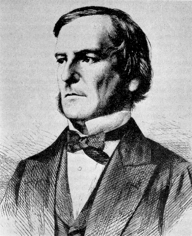
(1815-1864)
George Boole is the pioneer of the algebra we call Boolean algebra today. He introduced algebraic equations to express and manipulate logical propositions rigorously. The modern form of Boolean algebra serves as the primary mathematical tool for the design and analysis of digital circuits.
2.2.1. Axioms of Boolean Algebra
We bootstrap Boolean algebra by means of six axioms. Axioms have the form of equalities that we consider satisfied by definition. We postulate a digital domain of binary values \(\mathcal{B} = \{0, 1\},\) and three operations, AND (\(\cdot\)), OR (\(+\)), and NOT (overline \(\overline{\phantom{a}}\)). A Boolean variable represents a binary value, 0 or 1. Given Boolean variable \(x \in \mathcal{B},\) Table 2.1 lists the six axioms of Boolean algebra.
| Axiom | Dual Axiom | |
|---|---|---|
| Negation | \(\overline{0} = 1\) | \(\overline{1} = 0\) |
| Annihilation | \(x \cdot 0 = 0\) | \(x + 1 = 1\) |
| Identity | \(x \cdot 1 = x\) | \(x + 0 = x\) |
The negation axiom and its dual define the NOT operation. Negation excludes a third possibility: the negation of 0 is 1 and the negation of 1 is 0. The identity and annihilation axioms define the conjunction or AND operation. When it is clear from the context, we write the conjunction of Boolean variables \(x\) and \(y\) without the dot operator, such that \(x\,y = x \cdot y.\) Since Boolean variable \(x\) may assume value 0 or 1, each of the annihilation and identity axioms covers two cases that result in the following truth table, cf. AND Gate:
| \(x\) | \(y\) | \(x \cdot y\) | |
|---|---|---|---|
| 0 | 0 | 0 | by annihilation |
| 0 | 1 | 0 | by identity |
| 1 | 0 | 0 | by annihilation |
| 1 | 1 | 1 | by identity |
Analogously, the dual identity and annihilation axioms define the disjunction or OR operation, cf. OR Gate:
| \(x\) | \(y\) | \(x + y\) | |
|---|---|---|---|
| 0 | 0 | 0 | by identity |
| 0 | 1 | 1 | by annihilation |
| 1 | 0 | 1 | by identity |
| 1 | 1 | 1 | by annihilation |
The axioms and their duals are related through the principle of duality: If a Boolean equation is satisfied, then exchanging
- AND and OR operators, and
- 0’s and 1’s
yields a Boolean equation that is also satisfied. NOT operators remain unaffected by the principle of duality. To emphasize the distinction between an axiom and its dual, we also refer to the axiom as primal axiom. For example, applying the principle of duality to a dual axiom yields the primal axiom, which is the dual of the dual axiom.
In Boolean expressions with both AND and OR operators, AND has precedence over OR by convention. For example, \(x + y \cdot z\) means \(x + (y \cdot z)\) rather than \((x + y) \cdot z.\) If the association of operands and operators within an expression is unclear, we use explicit parenthesizations.
2.2.2. Switch Logic
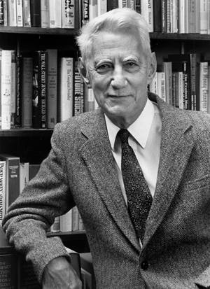
(1916-2001)
Claude Shannon discovered that Boolean algebra can be used to describe the behavior of electrical switching circuits. This insight earned him a master’s degree at MIT in 1937, and has been acclaimed as the most important master’s thesis of the \(20^{th}\) century.

Figure 2.1: Switch schematic (top) and compact form (bottom). The switch is closed if \(A = 1\) and open if \(A = 0.\)
In the following, we draw a switch compactly as two wire contacts around the signal name that controls the switch position, as shown in Figure 2.1. The switch connects or disconnects terminal nodes \(u\) and \(v.\) We assume that the switch is closed if the signal is 1 and open if the signal is 0. Thus, we may use Boolean variables, like \(A,\) to denote the control signal for the switch position. We introduce a switch function as an indicator of the switch position between nodes \(u\) and \(v\):
Since the switch position is a function of the control signal, we parameterize the switch function with the control signal. For the switch in Figure 2.1, the switch function is trivial:
If control signal \(A = 1,\) the switch is closed, and nodes \(u\) and \(v\) are connected. Otherwise, if \(A = 0,\) the switch is open, and nodes \(u\) and \(v\) are disconnected. This switch function models the behavior of an nMOS transistor with gate signal \(A.\)

Figure 2.2: A complemented switch is closed if \(A = 0\) and open if \(A = 1.\)
The complemented switch in Figure 2.2 models the behavior of a pMOS transistor with gate signal \(A.\) If control signal \(A = 0,\) the complemented control signal is \(\overline{A}=1.\) The switch is closed and nodes \(u\) and \(v\) are connected. Otherwise, if control signal \(A = 1,\) the complemented control signal is \(\overline{A}=0,\) the switch is open, and nodes \(u\) and \(v\) are disconnected. The switch function of the complemented switch is
The Boolean AND and OR operations enable us to analyze switch networks by deriving an equivalent switch, analogous to the equivalent resistor, see Section Resistor Networks, and equivalent capacitance, see Section Capacitor Networks of an electrical network. The basic compositions of two switches are the series and parallel composition. If we are given two switches controlled by Boolean variables \(A\) and \(B\) and compose the switches in series, then the terminal nodes \(u\) and \(v\) are connected if and only if both switches are closed, see Figure 2.3. If at least one of the switches is open, then the terminals are disconnected. Therefore, two switches in series can be represented by an equivalent switch whose control signal is the conjunction \(A\, B.\)

Figure 2.3: Series composition of switches (left) and equivalent switch with control signal \(A\,B\) (right).
We can derive the switch function of the series composition using a Boolean AND of the switch functions. Figure 2.3 on the left shows two uncomplemented switches with switch functions \(\sigma_{u,w}(A) = A\) and \(\sigma_{w,v}(B) = B.\) The conjunction yields the switch function of the series composition:
The switch function of the series composition expresses the connectivity of nodes \(u\) and \(v\) without reference to node \(w.\) In fact, inner node \(w\) is irrelevant for the abstract switch behavior between nodes \(u\) and \(v.\) This type of abstraction is key to modularization and hierarchical circuit design with subcircuits hidden in black boxes.
If we compose two switches controlled by Boolean variables \(A\) and \(B\) in parallel, then the terminals are disconnected if and only if both switches are open. If at least one switch is closed, then the terminals are connected. The equivalent switch is controlled by the disjunction \(A+B\) shown in Figure 2.4.

Figure 2.4: Parallel composition of switches (left) and equivalent switch with control signal \(A + B\) (right).
The switch function of the parallel composition of two uncomplemented switches with switch functions \(\sigma_{u,v}(A) = A\) and \(\sigma_{u,v}(B) = B\) is their disjunction:
The concept of an equivalent switch facilitates transforming a series-parallel switch network into a single switch controlled by a Boolean expression that represents the original switch network. Conversely, we may transform a switch with a Boolean expression for the control logic into a series-parallel switch network with Boolean variables to control the individual switches.

Figure 2.5: Example of a larger series-parallel switch network.
Consider the series-parallel switch network in Figure 2.5 with three parallel branches of two series switches each, controlled by Boolean variables \(A,\) \(B,\) and \(C.\) We analyze the switch network by transforming it into a single, equivalent switch, deriving the equivalent Boolean expression for the switch control in the process.
Figure 2.6 steps through the transformation process. First, we realize in Figure 2.5 that each of the three parallel branches consists of a series composition of two switches. Hence, we replace each of the series compositions with the corresponding equivalent switch, using an AND operation to form the control expressions \(A\,B,\) \(A\,C,\) and \(B\,C\) for the three branches. Figure 2.6 shows the resulting switch network on the left. Next, we consider the parallel composition of switches \(A\,B\) and \(A\,C.\) The parallel composition has an equivalent switch with an OR operation of the control expressions of the individual switches. The resulting switch network, shown in the middle of Figure 2.6, reduces the two parallel switches into a single switch with control logic \(A\,B + A\,C.\) The equivalent switch for the remaining parallel composition is shown on the right in Figure 2.6. The switch is controlled by the disjunction of \(A\,B + A\,C\) and \(B\,C,\) i.e. Boolean expression \((A\,B + A\,C) + B\,C.\)

Figure 2.6: Transformation of series-parallel switch network into an equivalent switch.
Note that we could have combined the parallel switches in the rightmost branches first. Then, we would have obtained Boolean expression \(A\,B + (A\,C + B\,C)\) with a different parenthesization. In fact, the order in which we transform the parallel compositions is immaterial, so that we can drop the parentheses altogether: \((A\,B + A\,C) + B\,C = A\,B + (A\,C + B\,C) = A\,B + A\,C + B\,C.\) Interactive Figure 2.7 enables you to explore the equivalent networks by selecting the values of Boolean variables \(A,\) \(B,\) and \(C.\)
A = 0 B = 0 C = 0 Figure 2.7: Interactive series-parallel switch network (left), equivalent switch (middle), and corresponding truth table (right).

Figure 2.8: Switch network with complemented and uncomplemented switches.
Switches can have different polarities. The uncomplemented switch of Figure 2.1 is closed if control signal \(A=1,\) whereas the complemented switch of Figure 2.2 is closed if control signal \(A=0.\) In a network where all switches under the control of one signal have the same polarity, the switch function is monotone in this signal. For example, if signal \(A\) controls uncomplemented switches only, then the switch function is monotonically increasing in \(A.\) This means that the network cannot connect previously disconnected terminals if \(A\) switches off, i.e. from 1 to 0. To implement any switch function we might be interested in, we generally need switches of both polarities.
Figure 2.8 shows a series-parallel switch network with complemented and uncomplemented switches. We can analyze the network analogous to Example 2.6, by transforming it into an equivalent switch. The resulting control signal obeys the Boolean expression
An alternative method for analyzing a switch network is the systematic enumeration of all combinations of input values of the control signals. For each input combination, we derive the value of the switch function by inspecting whether the terminals are connected or not. In case of Figure 2.8, switch function \(\sigma\) is a function of Boolean variables \(A,\) \(B,\) and \(C.\) The corresponding truth table enumerates all combinations of input values and the corresponding values of switch function \(\sigma(A,B,C)\):
\(A\) \(B\) \(C\) \(\sigma\) 0 0 0 0 0 0 1 1 0 1 0 1 0 1 1 0 1 0 0 1 1 0 1 0 1 1 0 0 1 1 1 1
Each row of the truth table defines one value of switch function \(\sigma(A,B,C)\) for the corresponding input values, that we deduce by inspecting the switch positions of the network. For example, if \(A=B=C=0,\) then the uncomplemented \(A\)-switch in the left half of network is open, so that the left half cannot connect the terminals, independent of the position of the \(B\)-switches and \(C\)-switches. In contrast, the complemented \(A\)-switch in the right half is closed when \(A=0,\) potentially connecting the terminals. However, neither of the lower parallel paths through the series of \(B\)-switches and \(C\)-switches closes if both \(B=0\) and \(C=0.\) Therefore, the terminals are disconnected for input combination \(A=B=C=0,\) and switch function \(\sigma(0,0,0)=0\) in the top row of the truth table. On the other hand, for input combination \(A=B=C=1,\) the three switches in the leftmost path of the network are closed and connect the terminals. Thus, switch function \(\sigma(1,1,1)=1\) in the bottom row of the truth table. The remaining rows can be derived analogously. The truth table specification and the Boolean expression of the switch function of a network are different yet equivalent forms. Both forms specify the 3-input XOR function. We show below how to transform one form into the other.
The truth table method applies to arbitrary switch networks, including non-series-parallel networks which we cannot transform into an equivalent switch by reducing series and parallel compositions. As an example, consider the network in Figure 2.9. This network is well known among electricians, because it is suited to control the lights in a stairway across three levels of a house. Each level has one light switch, for example the basement with control signal \(A,\) first floor with control signal \(B,\) and second floor with control signal \(C.\) Pushing any of the light switches will turn the lights either on or off. Each light switch contains two or four switches. You can add light switches to the network by including additional 4-way switches like the one controlled by input signal \(B\) with four terminals \(w,\) \(x,\) \(y,\) and \(z.\)

Figure 2.9: Non-series-parallel network: 3-input XOR suited for the control of stairway lights.
We analyze Figure 2.9 by constructing the truth table. Rather than inspecting the network for each of the eight input combinations of control signals \(A,\) \(B,\) and \(C,\) we save inspection effort by identifying only those input combinations that connect the terminals \(u\) and \(v\) and, therefore, have value \(\sigma(A,B,C)=1.\) The remaining rows of the table must have switch function value 0. More succinctly, we determine all simple paths that connect the terminals if all switches on the path are closed. Simple paths are paths that visit disjoint nodes only. The network has these simple paths between terminal nodes \(u\) and \(v,\) and associated values for control signals \(A,\) \(B,\) and \(C\) to close the path and connect the terminals:
simple path A B C \(u \rightarrow w \rightarrow x \rightarrow v\) 1 0 0 \(u \rightarrow w \rightarrow z \rightarrow v\) 1 1 1 \(u \rightarrow y \rightarrow z \rightarrow v\) 0 0 1 \(u \rightarrow y \rightarrow x \rightarrow v\) 0 1 0
The switch network has more simple paths than these four, including path \(u \rightarrow w \rightarrow z \rightarrow y \rightarrow x \rightarrow v.\) However, there exists no combination of control values to close the path, because it contains both complemented and uncomplemented switches controlled by input \(B.\) For example, if we choose \(B=1,\) then \(\sigma_{w,z}(B) = 1,\) but \(\sigma_{z,y}(B)=0,\) and the path does not connect terminals \(u\) and \(v.\) Otherwise, if \(B=0,\) then \(\sigma_{w,z}(B)=0\) and \(\sigma_{z,y}(B)=1,\) and the path does not connect the terminals either.
The network has even more paths between terminals \(u\) and \(v,\) such as path \(u \rightarrow w \rightarrow x \rightarrow y \rightarrow z \rightarrow w \rightarrow x \rightarrow v.\) However, this path is not simple, because it visits nodes \(w\) and \(x\) twice. Furthermore, the path cannot connect the terminals, because it contains both complemented and uncomplemented switches controlled by input \(B.\) To analyze a network, it suffices to find all simple paths between the nodes of interest. More complex paths cannot provide more connectivity information than simple paths capture already.
We translate our path analysis into a truth table by assigning a 1 to all input combinations that represent closed simple paths and 0 to all remaining input combinations. The resulting truth table is the same as for the switch network in Figure 2.8. We conclude that the non-series-parallel network in Figure 2.9 and the series-parallel network in Figure 2.8 implement the same switch function, a 3-input XOR function. The non-series-parallel network uses only eight switches compared to ten switches in the series-parallel network. This is no accident. Non-series-parallel implementations of symmetric switch functions are generally more compact than their equivalent series-parallel counterparts.
2.2.3. Theorems of Boolean Algebra
The theorems of Boolean algebra state properties of Boolean expressions in form of equalities. The proof method of choice for these theorems is perfect induction: enumerate all possible combinations of variable values and for each combination verify that the equality holds under the axioms of Boolean algebra.
We introduce the theorems of Boolean algebra starting with those theorems that involve a single Boolean variable \(A \in \mathcal{B}\):
Theorem Dual Theorem Idempotence \(A \cdot A = A\) \(A + A = A\) Complementation \(A \cdot \overline{A} = 0\) \(A + \overline{A} = 1\) Involution \(\overline{\overline{A}} = A\) \(\overline{\overline{A}} = A\)
If you remember one theorem you can apply the principle of duality to derive its dual theorem. Since NOT operators are unaffected by the principle of duality, the involution theorem and its dual are equal. We also denote a theorem as primal theorem when appropriate to emphasize that it is the dual of its dual theorem.
To illustrate the proof method of perfect induction, let us prove the complementation theorem. The complementation theorem states that the conjunction of \(A\) and its complement equals 0. Since Boolean variable \(A\) can assume two values 0 or 1, we construct a truth table with one row per value of \(A,\) and two columns, one for the left-hand side, lhs \(= A \cdot \overline{A},\) and the other for the right-hand side, rhs \(= 0,\) of equation \(A \cdot \overline{A} = 0\):
\(A\) lhs rhs 0 0 0 1 0 0
Since the rhs is equal to constant 0 independent of the value of \(A,\) we enter constant 0 in both rows of column rhs. The lhs of the theorem is a Boolean expression. A rigorous proof invokes the axioms of Boolean algebra to deduce the lhs values in each row. As the first case consider \(A = 0.\) The negation axiom yields \(\overline{A} = 1,\) so that \(A \cdot \overline{A} = 0 \cdot 1.\) Next, apply the identity axiom with \(x=0\) to obtain \(0 \cdot 1 = 0.\) Thus, we enter value 0 in the top row of the lhs column. Analogously, for \(A=1\) the negation axiom yields \(\overline{A}=0.\) Thus, the lhs is \(A \cdot \overline{A} = 1 \cdot 0.\) This conjunction has the form of the annihilation axiom. For \(x = 1,\) the identity axiom postulates that \(1 \cdot 0 = 0.\) Therefore, we enter value 0 in the bottom row of the lhs column. To complete the perfect induction we compare the columns of the lhs and the rhs row by row. Since the values are equal in all rows, we conclude that the equality holds, and the complementation theorem is proven.
When designing digital circuits, the theorems of Boolean algebra can be used to simplify a given circuit by removing gates. For example, the idempotence theorem, \(A \cdot A = A,\) and its dual, \(A + A = A,\) enable us to remove an AND gate or an OR gate such that input \(A\) remains as driver of the output wire:

Similarly, the complementation theorem, \(A \cdot \overline{A} = 0,\) and its dual, \(A + \overline{A} = 1,\) permit removing an AND gate or OR gate, and driving the output with 0 or 1 by tying the wire to GND or \(V_{DD}\):

The involution theorem, \(\overline{\overline{A}} = A,\) tells us that two back-to-back inverters can be removed without affecting the logical function. Simply drive the output wire with the input signal:

The design of a fast digital circuit may require adding rather than removing gates, with the goal to optimize the number of stages of a path. In this case, we can use the theorems of Boolean algebra in the opposite direction. For example, if we have a wire driven by input signal \(A,\) we can add two stages to the path by inserting two inverters. The involution theorem guarantees that the additional inverters do not change the logical function of the circuit.
The theorems of Boolean algebra with two and three Boolean variables \(A, B, C \in \mathcal{B}\) are:
Theorem Dual Theorem Commutativity \(A \cdot B = B \cdot A\) \(A + B = B + A\) Associativity \((A \cdot B) \cdot C = A \cdot (B \cdot C)\) \((A + B) + C = A + (B + C)\) Distributivity \(A \cdot (B + C) = (A \cdot B) + (A\cdot C)\) \(A + (B \cdot C) = (A + B) \cdot (A + C)\) Combining \((A \cdot B) + (A \cdot \overline{B}) = A\) \((A + B) \cdot (A + \overline{B}) = A\) Covering \(A \cdot (A + B) = A\) \(A + (A \cdot B) = A\) Absorption \(A \cdot (\overline{A} + B) = A \cdot B\) \(A + (\overline{A} \cdot B) = A + B\) De Morgan \(\overline{A \cdot B} = \overline{A} + \overline{B}\) \(\overline{A + B} = \overline{A} \cdot \overline{B}\)
It is straightforward to prove all of these theorems by means of perfect induction. As a representative example, we prove the absorption theorem \(A \cdot (\overline{A} + B) = A \cdot B.\) This theorem reduces the size of the left-hand side by absorbing the complement of \(A.\) Since the theorem involves two variables, \(A\) and \(B,\) the truth table for the perfect induction comprises four rows, one for each of the combinations \(A\,B \in \{ 00, 01, 10, 11\}.\) The right-hand side of the theorem, rhs \(= A \cdot B,\) is simpler than the left-hand side, lhs \(= A \cdot (\overline{A} + B).\) Therefore, we prove the lhs in three steps, and include separate columns for subexpressions \(\overline{A}\) and \(\overline{A} + B.\)
\(A\) \(B\) \(\overline{A}\) \(\overline{A} + B\) lhs rhs 0 0 1 1 0 0 0 1 1 1 0 0 1 0 0 0 0 0 1 1 0 1 1 1
Column \(\overline{A}\) negates the values in column \(A\) by the negation axiom. The column for the rhs is derived from the AND operation \(A \cdot B\) that we proved with the axioms of Boolean algebra for \(x=A\) and \(y=B\) already. Subexpression \(\overline{A}+B\) is the disjunction of the values in the column for \(\overline{A}\) and the column for \(B.\) Thus, we rely on the proof of the OR operation with the axioms of Boolean algebra to deduce that \(\overline{A} + B\) is 0 only if \(\overline{A} = 0\) and \(B=0,\) which is true in the third row of the table. Analogously, the lhs is a conjunction of the values in the columns for \(A\) and \(\overline{A} + B.\) We deduce the values in the lhs column by noting that the conjunction is 1 only if \(A=1\) and \(\overline{A} + B = 1,\) which is true in the bottom row of the table. We conclude the perfect induction by noting that the columns for the lhs and the rhs are identical, which proves the absorption theorem.
Perfect induction is a brute-force proof method that works well for theorems with one or two variables. With three variables, the truth table has eight rows already, increasing the chances of error during the manual construction process. The theorems of Boolean algebra empower us to prove the equality of Boolean expressions by algebraic manipulation. This method starts with one side of the equation, and deduces the other side by repeated application of the theorems of Boolean algebra. As an example, we offer an alternative proof of the absorption theorem by means of Boolean algebra:
Using three of the theorems of Boolean algebra and the identity axiom, we have transformed the lhs of the absorption theorem into the rhs. The opposite direction constitutes a valid proof too, because equalities hold independent of the direction of the derivation. With a little practice and a good command of the theorems of Boolean algebra, we can often construct proofs by Boolean algebra that are shorter and clearer than the equivalent proofs by perfect induction.
Prove these theorems by perfect induction:
- combining theorem: \(A \cdot B + A \cdot \overline{B} = A,\)
- covering theorem: \(A \cdot (A + B) = A.\)
Both theorems involve two Boolean variables \(A\) and \(B.\) Therefore, we construct truth tables with four rows, one row per combination of input values \(A B = \{ 00, 01, 10, 11\}.\)
We begin with the perfect induction of combining theorem \(A \cdot B + A \cdot \overline{B} = A.\) The right-hand side rhs \(= A\) is trivial: it is a copy of the column of variable \(A.\) The left-hand side is a disjunction of conjunctions. We introduce three columns for its subexpressions: one column for \(\overline{B},\) and one column for conjunctions \(A \cdot B\) and \(A \cdot \overline{B}\) respectively.
| \(A\) | \(B\) | \(\overline{B}\) | \(A \cdot B\) | \(A \cdot \overline{B}\) | lhs | rhs |
|---|---|---|---|---|---|---|
| 0 | 0 | 1 | 0 | 0 | 0 | 0 |
| 0 | 1 | 0 | 0 | 0 | 0 | 0 |
| 1 | 0 | 1 | 0 | 1 | 1 | 1 |
| 1 | 1 | 0 | 1 | 0 | 1 | 1 |
Column \(\overline{B}\) is a direct consequence of the negation axioms. In each row where \(B = 0,\) insert the complement \(\overline{B} = 1,\) and where \(B = 1,\) insert \(\overline{B} = 0.\) Column \(A \cdot B\) equals 1 only in the row where both \(A\) and \(B\) are 1, which is the bottom row of the truth table. Analogously, column \(A \cdot \overline{B}\) equals 1 only in the row where \(A\) and \(\overline{B}\) are 1, i.e. in the third row. The left-hand side is the disjunction of the columns for \(A\cdot B\) and \(A\cdot \overline{B}.\) The disjunction is 0 only in those rows where both subexpressions \(A\cdot B = 0\) and \(A\cdot \overline{B} = 0,\) which are the two top rows in the table. Comparing the columns of lhs and rhs, we find that the columns are equal, which proves the combining theorem.
Next, we prove the covering theorem by perfect induction. Again, the rhs is simply a copy of the column of variable \(A.\) The lhs \(A \cdot (A + B)\) is a conjunction of \(A\) and disjunction \(A+B.\) Thus, we introduce a separate column for subexpression \(A+B.\)
| \(A\) | \(B\) | \(A + B\) | lhs | rhs |
|---|---|---|---|---|
| 0 | 0 | 0 | 0 | 0 |
| 0 | 1 | 1 | 0 | 0 |
| 1 | 0 | 1 | 1 | 1 |
| 1 | 1 | 1 | 1 | 1 |
The disjunction \(A + B\) is 0 only where both variables \(A\) and \(B\) are 0, which is in the first row only. The lhs is 1 only where both \(A\) and \(A+B\) are 1, which is the case in the two bottom rows. We conclude that the covering theorem is proven, because the columns for lhs and rhs are equal.
2.2.4. Normal Forms
Equality is an important relation of two switch networks. Given two switch networks, their analysis should reveal unambiguosly whether the networks are functionally equal because they implement the same switch function or not. This knowledge enables the circuit designer to choose the smaller, faster, or less expensive design. For example, the switch networks in Figure 2.8 and Figure 2.9 have the same switch function, because our analysis revealed that both networks have the same truth table. Network analysis by deriving a truth table is essentially a proof by perfect induction. In this section we discuss an alternative style of analysis based on Boolean algebra. In short, every Boolean expression has a unique canonical or normal form. If we are given two Boolean expressions, we can prove their equality by transforming each into normal form. If the normal forms are identical, then the Boolean expressions are equal.
The combining theorems of Boolean algebra are the key to deriving a normal form of a Boolean expression. The combining theorem, \((A \cdot B) + (A \cdot \overline{B}) = A,\) and its dual, \((A + B) \cdot (A + \overline{B}) = A,\) eliminate one variable, \(B,\) from an expression in two variables, \(A\) and \(B.\) Here is the proof of the combining theorem with lhs \(= (A \cdot B) + (A \cdot \overline{B})\) and rhs \(= A\) by perfect induction:
\(A\) \(B\) \(\overline{B}\) \(A \cdot B\) \(A \cdot \overline{B}\) lhs rhs 0 0 1 0 0 0 0 0 1 0 0 0 0 0 1 0 1 0 1 1 1 1 1 0 1 0 1 1
If we use the combining theorem to include rather than eliminate Boolean variables, we arrive at a normal form. Given a set of Boolean variables, and a Boolean expression, we apply the combining theorem repeatedly until each conjunction contains all Boolean variables in complemented or uncomplemented form. This construction process terminates for a finite number of Boolean variables. For example, if we are given a Boolean expression \(\overline{A} + B\) in two variables, \(A\) and \(B,\) we apply the combining theorem to each operand of the disjunction and remove duplicate conjunctions by virtue of the idempotence theorem:
Boolean expression \(\overline{A}\,B + \overline{A}\,\overline{B} + A\,B\) is a so-called sum-of-products normal form, abbreviated SOP normal form, because it is a disjunction (sum) of conjunctions (products), and each conjunction contains all variables either in complemented or uncomplemented form.
The fact that an SOP is unique follows immediately from the associated truth table representation. The truth table below proves the equality \(\overline{A}\,B + \overline{A}\,\overline{B} + A\,B = \overline{A} + B\) by perfect induction.
\(A\) \(B\) \(\overline{A}\,B\) \(\overline{A}\,\overline{B}\) \(A\,B\) \(\overline{A}\,B + \overline{A}\,\overline{B}+ A\,B\) \(\overline{A} + B\) 0 0 0 1 0 1 1 0 1 1 0 0 1 1 1 0 0 0 0 0 0 1 1 0 0 1 1 1
The equality proof itself is not of primary interest here, although it confirms our earlier derivation by Boolean algebra. Instead, we focus our attention on the three columns for the conjunctions \(\overline{A}\,B,\) \(\overline{A}\,\overline{B},\) and \(A\,B\) of the SOP normal form. Observe that each of these three columns contains exactly one 1. All other entries are 0. This is no accident. Each combination of input values in a row of the truth table corresponds to exactly one unique conjunction of all Boolean variables in complemented or uncomplemented form. If the variable value in a row is 1, the variable appears in uncomplemented form in the conjunction, and if the variable value is 0 the variable appears in complemented form. These conjunctions are called minterms. For two Boolean variables there are four minterms, each with value 1 only for the variable values in the associated row:
decimal \(A\) \(B\) minterm 0 0 0 \(\overline{A}\,\overline{B}\) 1 0 1 \(\overline{A}\,B\) 2 1 0 \(A\,\overline{B}\) 3 1 1 \(A\,B\)
If we interpret the juxtaposition of the Boolean variable values as an unsigned binary number, each row is associated with a unique number. The table above includes the numbers in decimal format in the leftmost column. Thus, we may refer to a minterm by its associated decimal number. Then, the SOP normal form can be written as a disjunction (sum) of those minterms for which the function is 1. For example, we may write our SOP normal form with decimal minterm codes as:
The sorted list of minterm codes in the sum identifies the switch function in a syntactically unique form. It lists all rows of the truth table where the function assumes value 1. Two switch functions are equal if and only if they have the same sorted list of minterms. Comparing two lists of minterms is equivalent to comparing two columns of a truth table during a perfect induction.
We conclude that a truth table and a SOP normal form are isomorphic specifications of a switch function. More generally, switch function \(f(x_0, x_1, \ldots, x_{n-1})\) in \(n\) Boolean variables \(x_0, x_1, \ldots, x_{n-1}\) can be specified by means of a truth table with \(2^n\) rows with combinations of variable values in decimal range \([0,2^n-1].\) In the column for switch function \(f \in \mathcal{B}\) we assign either Boolean value 0 or 1 to the value combination in each row. The isomorphic specification of switch function \(f\) by means of an SOP normal form is the disjunction of up to \(2^n\) minterms in range \([0,2^n-1]\) for which \(f\) assumes value 1.
We may derive the SOP normal form of a switch function \(f(x_0, x_1, \ldots, x_{n-1})\) rigorously from a truth table specification by factoring \(f\) about each of the variables with the aid of Shannon’s expansion theorem:
This equation expands \(f\) about variable \(x_0.\) The expansions about any of the other variables look analogously. The expansion theorem tells us that \(f\) can be written as a disjunction of two conjunctions. In the first conjunction, we replace all occurrences of \(x_0\) in \(f\) with constant 0, and AND the resulting expression with \(\overline{x}_0.\) Similarly, the second conjunction substitutes constant 1 for all occurrences of \(x_0\) in \(f,\) and ANDs the result with \(x_0.\) Note that variable \(x_0\) vanishes out of expressions \(f(0, x_1, \ldots, x_{n-1})\) and \(f(1, x_1, \ldots, x_{n-1}).\) We may view Shannon’s expansion as an operation that lifts variable \(x_0\) out of \(f\) into the top-level disjunction. There, \(x_0\) acts like the predicate of the ite function, or the select input of a multiplexer.
Shannon’s expansion theorem is quickly proven by perfect induction, even without constructing a truth table: The Shannon expansion about Boolean variable \(x_0\) can take one of two forms, depending on the value of \(x_0.\) For \(x_0 = 0,\) Shannon’s expansion theorem yields equation:
Otherwise, for \(x_0 = 1,\) Shannon’s expansion theorem states:
Since the equations for each of the two cases are true statements, the theorem is proven.
Now, apply the Shannon expansion to each of the variables of switch function \(f\):
which is the SOP normal form of \(f,\) given the function values for all combinations of variable values.
For example, our Boolean expression \(\overline{A} + B\) specifies a switch function in two variables \(f(A,B) = \overline{A} + B,\) that expands to
We tabulate the evaluation of \(f(A,B)\) for all combinations of variable values to stress the isomorphism with the corresponding truth table:
decimal \(A\) \(B\) \(f(A,B) = \overline{A}+B\) 0 0 0 \(f(0,0) = 1\) 1 0 1 \(f(0,1) = 1\) 2 1 0 \(f(1,0) = 0\) 3 1 1 \(f(1,1) = 1\)
Substituting these function values into the Shannon expansion, we obtain the SOP normal form of \(f\):
Shannon’s expansion theorem is famous in parts because it provides a clean mathematical connection between a truth table and the corresponding SOP normal form.
The principle of duality points us to another normal form, the product-of-sums normal form, or POS normal form for short. We may use the dual combining theorem, \((A + B) \cdot (A + \overline{B}) = A,\) to include all variables of a switch function in each disjunction. Disjunctions that include all variables of a switch function in complemented or uncomplemented form are called maxterms. For example, assume we are given function \(f(A,B) = \overline{A} \cdot B.\) Application of the dual combining theorem and subsequent removal of duplicate disjunctions yields the corresponding POS normal form of \(f\):
The general construction procedure of the POS normal form relies on the dual of Shannon’s expansion theorem:
to expand function \(f\) about all variables:
Given the function values of \(f\) for all combinations of variable values, we obtain the POS normal form. If the function value is 1, then the associated maxterm vanishes from the POS due to the identity and dual annihilation axioms. Otherwise, if the function value is 0, the associated maxterm is included in the POS by virtue of the dual identity axiom.
The maxterms and function values of switch function \(f(A,B) = \overline{A} \cdot B\) are listed in the truth table:
decimal \(A\) \(B\) maxterm \(f(A,B) = \overline{A} \cdot B\) 0 0 0 \(A + B\) \(f(0,0) = 0\) 1 0 1 \(A + \overline{B}\) \(f(0,1) = 1\) 2 1 0 \(\overline{A} + B\) \(f(1,0) = 0\) 3 1 1 \(\overline{A} + \overline{B}\) \(f(1,1) = 0\)
Substituting these function values in the dual Shannon expansion, we obtain the POS normal form:
The product of the sorted list of decimal maxterm codes is a unique normal form of the switch function.
The SOP and POS normal forms of a switch function are logically equal, but are not duals of each other in general. For example, function \(f(A,B)=\overline{A}+B\) has SOP and POS normal forms:
In fact, function \(\overline{A} + B\) is in POS normal form already, because the expression is equal to maxterm 2. Similarly, function \(f(A,B)=\overline{A}\cdot B\) has SOP and POS normal forms:
Boolean expression \(\overline{A} \cdot B\) is in SOP normal form already, because it equals minterm 1. For neither switch function are the SOP and POS normal forms duals of each other, because the number of minterms and maxterms differ. However, the normal forms of a function are related through the sets of minterm and maxterm codes. The sets of minterm codes of the SOP normal form and maxterm codes of the POS normal form of a switch function in \(n\) variables are disjoint, and their union is the complete set of codes \(\{0,1, \ldots, 2^n-1\},\) i.e. the sets are partitions of code set \(\{0,1,\ldots,2^n-1\}.\) A longer SOP normal form implies a shorter POS normal form in terms of the length of the lists of minterms and maxterms and vice versa. We may exploit this fact by choosing the shorter normal form to specify a switch function.
The names minterm and maxterm may have originated in the following analogy. Consider the algebraic order of the numbers in \(\mathcal{B} = \{0, 1\},\) where the common relation \(0 < 1\) holds. Therefore, given two Boolean variables \(A, B \in \mathcal{B},\) then the conjunction is equivalent to the minimum and the disjunction to the maximum, i.e. these identies hold:
Here are the proofs by perfect induction:
\(A\) \(B\) \(A \cdot B\) \(\min(A, B)\) \(A + B\) \(\max(A, B)\) 0 0 0 0 0 0 0 1 0 0 1 1 1 0 0 0 1 1 1 1 1 1 1 1
The conjunction of \(A\) and \(B\) is 1 only if both \(A\) and \(B\) are 1. Analogously, the minimum of \(A\) and \(B\) is 1 only if both \(A\) and \(B\) are 1. The disjunction of \(A\) and \(B\) is 0 only if both \(A\) and \(B\) are 0. Analogously, the maximum of \(A\) and \(B\) is 0 only if both \(A\) and \(B\) are 0.
This analogy may also help to remember the structure of the normal forms. Since a SOP may be viewed as the maximum-of-minima, a SOP assumes value 1 if one of its minterms is 1. Analogously, a POS can be viewed as the minimum-of-maxima. Hence, a POS assumes value 0 if one of its maxterms is 0.
Use the Shannon expansion to derive the SOP normal form for
- \(f(x,y) = x + y,\)
- \(g(x,y) = x \cdot y.\)
We expand \(f(x,y)\) about its variables \(x\) and \(y\) without any simplifications other than localized applications of the annihilation and identity axioms. This is an important restriction, because our goal is to expand rather than to reduce \(f.\) First, we expand \(f\) about \(x\):
\[\begin{eqnarray*} x + y &=& \overline{x} \cdot (x + y)|_\overline{x} + x \cdot (x + y)|_x \\ &=& \overline{x} \cdot (0 + y) + x \cdot (1 + y) \\ &=& \overline{x}\,y + x\,1 \\ &=& \overline{x}\,y + x\,. \end{eqnarray*}\]We continue by expanding the result about \(y\):
\[\begin{eqnarray*} x + y &=& \overline{y} \cdot (\overline{x}\,y + x)|_\overline{y} + y \cdot (\overline{x}\,y + x)|_y \\ &=& \overline{y} \cdot (\overline{x} \cdot 0 + x) + y \cdot (\overline{x} \cdot 1 + x) \\ &=& \overline{y} \cdot x + y \cdot (\overline{x} + x) \\ &=& x\,\overline{y} + \overline{x}\,y + x\,y\,. \end{eqnarray*}\]We find Boolean expression \(x\,\overline{y} + \overline{x}\,y + x\,y,\) which is the SOP normal form of \(x+y\) with three minterms.
We procede analogously to (a), starting to expand \(g\) about \(x\):
\[\begin{eqnarray*} x \cdot y &=& \overline{x} \cdot (x \cdot y)|_\overline{x} + x \cdot (x \cdot y)|_x \\ &=& \overline{x} \cdot (0 \cdot y) + x \cdot (1 \cdot y) \\ &=& 0 + x \cdot y \\ &=& x\,y\,. \end{eqnarray*}\]Next we expand the result about \(y\):
\[\begin{eqnarray*} x \cdot y &=& \overline{y} \cdot (x\,y)|_\overline{y} + y \cdot (x\,y)|_y \\ &=& \overline{y} \cdot (x \cdot 0) + y \cdot (x \cdot 1) \\ &=& 0 + y \cdot x \\ &=& x\,y\,. \end{eqnarray*}\]Boolean expression \(x\,y\) is the SOP normal form of \(x \cdot y.\) We realize that \(g(x,y) = x \cdot y\) has been given in SOP normal form already.
The XNOR function \(f_9\) and implication \(f_{11}\) are specified in this truth table:
| \(x\) | \(y\) | \(f_9\) | \(f_{11}\) |
|---|---|---|---|
| 0 | 0 | 1 | 1 |
| 0 | 1 | 0 | 1 |
| 1 | 0 | 0 | 0 |
| 1 | 1 | 1 | 1 |
- Derive the SOP normal forms of \(f_9\) and \(f_{11}\) from the truth table.
- Draw the gate-level circuits corresponding to the SOP normal forms.
- Derive the POS normal forms of \(f_9\) and \(f_{11}\) from the truth table.
- Draw the gate-level circuits corresponding to the POS normal forms.
The SOP normal form is the sum (logical OR) of the minterms where function \(f = 1.\) We begin with Boolean function \(f_9.\) According to the truth table, \(f_9 = 1\) in the first and forth row. The corresponding minterms are \(\overline{x}\,\overline{y}\) and \(x\,y.\) Thus, the SOP normal form of \(f_9\) is their sum (disjunction):
\[f_9 = \overline{x}\,\overline{y} + x\,y\,.\]Function \(f_{11}\) has three rows in the truth table where \(f_{11} = 1.\) The minterm corresponding to the first row is \(\overline{x}\,\overline{y},\) the minterm of the second row is \(\overline{x}\,y,\) and of the forth row \(x\,y.\) The SOP normal form of \(f_{11}\) is the sum (disjunction) of these minterms:
\[f_{11} = \overline{x}\,\overline{y} + \overline{x}\,y + x\,y\,.\]Every SOP normal form can be implemented with one AND gate per minterm and one OR gate that combines the outputs of the AND gates. The resulting circuits are classified as two-level circuits, and assume that input signals are available in complemented and uncomplemented form. If this is not the case, you need additional inverters. Here are the gate-level schematics for Boolean functions \(f_9\) and \(f_{11}\):

The POS normal form is the product (logical AND) of the maxterms where function \(f = 0.\) In the truth table for Boolean function \(f_9,\) we find that \(f_9 = 0\) in the second and third row. The maxterm of the second row is \(x + \overline{y}\) and the maxterm of the third row \(\overline{x} + y.\) The POS normal form is the product (conjunction) of these maxterms:
\[f_9 = (x + \overline{y}) \cdot (\overline{x} + y)\,.\]Function \(f_{11}\) has only one row with function value 0, the third row of the truth table. The corresponding maxterm is \(\overline{x} + y.\) The POS normal form consists of this maxterm only, no product is required for one maxterm:
\[f_{11} = \overline{x} + y\,.\]Every POS normal form can be implemented with one OR gate per maxterm and one AND gate that combines the outputs of the OR gates. The case of a single maxterm is a special case, where no AND gate is required, and the circuit has only one level rather than the common two-level circuits.

2.2.5. Boolean Functions
The use of switch functions as indicators of a switch position and their manipulation with the theorems of Boolean algebra has led to switching theory as an independent branch of mathematical study. To emphasize their relevance beyond circuits, switch functions are synonymously called Boolean functions. A Boolean function \(f:\mathcal{B}^n \rightarrow \mathcal{B}\) in \(n\) variables \(x_0, x_1, \ldots, x_{n-1}\) assigns to each point \((x_0, x_1, \ldots, x_{n-1}) \in \mathcal{B}^n\) a value \(f(x_0, x_1, \ldots, x_{n-1}) \in \mathcal{B}.\) For a given number of variables \(n > 0,\) \(\mathcal{B}^n\) comprises \(2^n\) unique points and associated function values. Since each of the \(2^n\) function values in \({B}\) can assume one of two values, the number of Boolean functions in \(n\) variables is \(2^{2^n}.\) For example, Table 2.2 lists all Boolean functions in \(n=2\) variables \(x\) and \(y.\) Index \(i\) of function \(f_i(x,y)\) is the decimal value of the function values interpreted as 4-bit binary number with the LSB in the top row. Although the number of Boolean functions is finite, we can construct infinitely many Boolean expressions that represent one Boolean function.
| \(x\) | \(y\) | \(f_0\) | \(f_1\) | \(f_2\) | \(f_3\) | \(f_4\) | \(f_5\) | \(f_6\) | \(f_7\) | \(f_8\) | \(f_9\) | \(f_{10}\) | \(f_{11}\) | \(f_{12}\) | \(f_{13}\) | \(f_{14}\) | \(f_{15}\) |
|---|---|---|---|---|---|---|---|---|---|---|---|---|---|---|---|---|---|
| 0 | 0 | 0 | 1 | 0 | 1 | 0 | 1 | 0 | 1 | 0 | 1 | 0 | 1 | 0 | 1 | 0 | 1 |
| 0 | 1 | 0 | 0 | 1 | 1 | 0 | 0 | 1 | 1 | 0 | 0 | 1 | 1 | 0 | 0 | 1 | 1 |
| 1 | 0 | 0 | 0 | 0 | 0 | 1 | 1 | 1 | 1 | 0 | 0 | 0 | 0 | 1 | 1 | 1 | 1 |
| 1 | 1 | 0 | 0 | 0 | 0 | 0 | 0 | 0 | 0 | 1 | 1 | 1 | 1 | 1 | 1 | 1 | 1 |
The Boolean functions in two variables appear in various contexts. Besides being the primary subject of study in areas like formal logic, we implement Boolean functions as logical operations in digital circuits to perform computations. Table 2.3 lists for each of the Boolean functions in two variables a Boolean expression and commonly used names.
| Function | Expression | Name(s) |
|---|---|---|
| \(f_0\) | 0 | constant 0, contradiction |
| \(f_1\) | \(\overline{x + y}\) | NOR, nondisjunction |
| \(f_2\) | \(\overline{x}\,y\) | \(<\), converse nonimplication |
| \(f_3\) | \(\overline{x}\) | left NOT, left complementation |
| \(f_4\) | \(x\,\overline{y}\) | \(>\), nonimplication |
| \(f_5\) | \(\overline{y}\) | right NOT, right complementation |
| \(f_6\) | \(\overline{x}\,y + x\,\overline{y}\) | XOR, inequality |
| \(f_7\) | \(\overline{x\,y}\) | NAND, nonconjunction |
| \(f_8\) | \(x\,y\) | AND, conjunction |
| \(f_9\) | \(x\,y + \overline{x}\,\overline{y}\) | XNOR, equality |
| \(f_{10}\) | \(y\) | right projection |
| \(f_{11}\) | \(\overline{x} + y\) | \(\le\), implication |
| \(f_{12}\) | \(x\) | left projection |
| \(f_{13}\) | \(x + \overline{y}\) | \(\ge\), converse implication |
| \(f_{14}\) | \(x + y\) | OR, disjunction |
| \(f_{15}\) | 1 | constant 1, tautology |
Four of the two-variable functions are trivial, \(f_0(x,y) = 0\) and \(f_{15}(x,y) = 1\) are constant, and \(f_{12}(x,y) = x\) and \(f_{10}(x,y) = y\) are the projections or selection operations. No transistors are required to implement these functions within a CMOS circuit.
Functions \(f_3(x,y) = \overline{x}\) and \(f_5(x,y) = \overline{y}\) require an inverter to compute the complemented projections. If we interpret the Boolean values 0 and 1 as numbers, we may express the complement as the arithmetic difference \(\overline{x} = 1 - x.\)
The NOR function \(f_1(x,y) = \overline{x + y}\) and NAND function \(f_7(x,y) = \overline{x\,y}\) require four transistors each to implement a NOR gate and a NAND gate. With an additional inverter at the output, we can implement the AND function \(f_8(x,y) = x\,y\) and the OR function \(f_{14}(x,y) = x + y\) as AND gate and OR gate, respectively. When interpreting 0 and 1 as numbers, we can interpret the AND function as arithmetic multiplication. We might be tempted to interpret the OR function as arithmetic addition. However, then \(f_{14}(1,1) = 1 + 1\) has value 2, which is not a Boolean value. In fact, the OR function is quite tricky when interpreted as arithmetic operation. You may want to proof that \(f_{14}\) can be expressed arithmetically as \(x + (1-x)\,y,\) which is equivalent to Boolean expression \(x + \overline{x}\,y.\) The latter is equal to \(f_{14}\) by absorption.
Four of the Boolean functions may be viewed as algebraic order relations, \(f_2(x,y) = \overline{x}\,y = x < y,\) \(f_4(x,y) = x\,\overline{y} = x > y,\) \(f_{11}(x,y) = \overline{x} + y = x \le y,\) and \(f_{13}(x,y) = x + \overline{y} = x \ge y,\) when interpreting Boolean values 0 and 1 as numbers. The less than relation \(f_2\) on numbers 0 and 1 is true only in case \(x=0\) and \(y=1,\) i.e. \(0 < 1,\) and is false in all other cases. Similarly, the greater than relation \(f_4\) is true for \(1 > 0\) only. The less than or equal relation \(f_{11}\) is false if \(x=1\) and \(y=0\) only, i.e. \(1 \not\le 0.\) Similarly, the greater than or equal relation \(f_{13}\) is false only in case \(0 \not\ge 1.\)
If we interpret Boolean values 0 and 1 as truth values False and True, then we observe another analogy to formal logic. Function \(f_{11}\) may be interpreted as logical implication \(f_{11}(x,y) = x \Rightarrow y.\) Premise \(x\) implies conclusion \(y\) if \(x\) is True and \(y\) is True. A False premise \(x\) implies anything, including a True or False conclusion \(y.\) Analogously, function \(f_{13}\) may be interpreted as converse implication \(y \Rightarrow x,\) and \(f_2\) and \(f_4\) are the complemented implications, or nonimplications, \(f_2 = \overline{f}_{13}\) and \(f_4 = \overline{f}_{11}.\) The CMOS circuits for \(f_2,\) \(f_4,\) \(f_{11},\) and \(f_{13}\) require six transistors each, one inverter to complement one of the inputs followed by a four-transistor CMOS gate.
The two remaining functions the XOR function \(f_6(x,y) = x \oplus y\) and XNOR function \(f_9(x,y) = \overline{x \oplus y},\) here written with operator symbol \(\oplus.\) The CMOS implementations of the XOR gate and the XNOR gate require twelve transistors each, two inverters to complement the inputs plus an eight-transistor CMOS gate. The exclusive XOR and the inclusive OR are related through the AND function:
The XOR function contributes two minterms and the AND function the third minterm to the inclusive OR function. If we interpret Boolean values 0 and 1 as truth values False and True, we observe that the XNOR function is True if and only if \(x = y,\) and the XOR function is True if and only if \(x \ne y.\) Thus, we may interpret the XNOR function as equality and the XOR function as inequality. In formal logic, it is also common to denote XNOR as equivalence and XOR as nonequivalence. The XOR function has another useful interpretation. If we interpret the Boolean values 0 and 1 as numbers, then the XOR is also a modulo-2 addition:
The XOR function has countless number-theoretical applications including cryptographic computations.
Beyond the Boolean functions in two variables, a handful of the \(2^{2^3} = 256\) functions in three variables deserve our attention, because they occur frequently in the design of digital circuits and because they are delightful on their own right. We introduce the parity, majority, and if-then-else function.
The three-variable parity function, \(P: \mathcal{B}^3 \rightarrow \mathcal{B},\) is:
Parity \(P\) equals 1 if the number of 1-inputs is odd. To be precise, \(P\) is the odd parity function. Negation of \(P\) yields the even parity function, which is 1 if the number of 1-inputs is even. The parity function is a basic operation in digital circuits, for example to compute the sum output of a full adder.
The parity function facilitates error detection in digital communication and storage systems, where individual bits may flip due to physical failure or sabotage. For example, assume we wish to send three bits, 101, to a receiver. Rather than transmitting these three bits, we compute the parity bit, \(P(1,0,1) = 0,\) append it to the three data bits, and transmit the resulting 4-bit packet 1010 to the receiver. The receiver can compute the parity of the first three bits and compare it with the fourth parity bit to detect an error. If the transmission is correct, then the receiver finds that \(P(1,0,1) = 0\) equals the parity bit, and concludes that all four bits are correct. If one of the data bits flips during the transmission, we may receive data bits 001, 111, or 100 rather than 101. Now, parity \(P(0,0,1) = P(1,1,1) = P(1,0,0) = 1\) differs from parity bit 0. The receiver detects the error and may request a retransmission. The same conclusion applies if the parity bit itself flips during the transmission. Unfortunately, the parity bit is not capable of detecting two bit flips. For example, if we receive data bits 110, then parity \(P(1,1,0) = 0\) equals the parity bit of the original data 101, and we become victims of a false positive if we conclude the received data are correct. More elaborate coding schemes than the simple parity check can be used to handle multiple bit flips.
The three-variable majority function, \(M: \mathcal{B}^3 \rightarrow \mathcal{B},\) is:
As the name suggests, \(M\) returns the majority value of three Boolean values. If more than half the values are 1 then \(M=1.\) The majority function serves as a basic operation in digital circuits, for instance to compute the carry output of a full adder. Besides such mundane uses, the majority function has some astonishing properties. We briefly discuss a connection to graph theory.[3]
If we interpret variables \(x,\) \(y,\) and \(z\) of \(M\) as numbers, conjunction as min and disjunction as max function, then the majority function can be viewed as the median, \(M(x,y,z) = y\) if \(x \le y \le z,\) such that \(M(0,0,0) = M(0,0,1) = 0\) and \(M(0,1,1) = M(1,1,1) = 1.\) This interpretation holds not only for numbers 0 and 1, but also if \(x,\) \(y,\) and \(z\) are arbitrary real numbers. We can define a median algebra with three axioms on a set of numbers, e.g. with \(w, x, y, z \in \{0, 1\}\):
Name Axiom Majority \(M(x,x,y) = x\) Commutativity \(M(x,y,z) = M(x,z,y) = M(y,x,z) = M(y,z,x) = M(z,x,y) = M(z,y,x)\) Associativity \(M(x,w,M(y,w,z)) = M(M(x,w,y),w,z)\)
Given \(u\) and \(v\) in \(\{0, 1\},\) then function \(g(x) = M(x,u,v)\) can be shown to satisfy
and \(g\) is a homomorphism. We can use function \(g\) to compute for each vertex of a free tree a median label. Given vertex \(x\) and a tree edge \((u,v),\) project \(x\) to vertex \(u\) if \(u\) is closer to \(x\) than \(v,\) otherwise project \(x\) to \(v.\) This example illustrates the projection:

For example, vertex \(a\) is closer to \(c\) than to \(e.\) Therefore, we project \(a\) to vertex \(c\) of edge \((c,e).\) Each such projection is a homomorphism. The bit strings on the right are the binary encoded labels of the vertices, e.g. label \(L(f) = 1001100,\) assuming arbitrarily that \(L(a) = 0000000.\) Hence, vertex \(a\) of edge \((a,c)\) is encoded with 0, and vertex \(c\) with 1. The vertex labels enable us to compute the median of three vertices of the tree by computing the medians of each component of the labels. For example, the median of vertices \(e,\) \(g,\) and \(h\) is vertex \(f,\) because the bitwise median of \(L(e) = 1001000,\) \(L(g) = 1001110,\) and \(L(h) = 1001101\) is \(1001100 = L(f).\) Analogously, the median of vertices \(c,\) \(e,\) and \(f\) is vertex \(e,\) because the bitwise median of \(L(c) = 1000000,\) \(L(e) = 1001000,\) and \(L(f) = 1001100\) is \(1001000 = L(e),\) confirming that \(e\) is the center of \(c,\) \(e,\) and \(f.\) Amazing what majority can do for us, isn’t it!
The if-then-else function, or ite for short, is a three-variable function \(ite: \mathcal{B}^3 \rightarrow \mathcal{B},\) defined as:
The ite function equals \(t\) if \(p = 1\) and \(e\) if \(p=0.\) This behavior is the logical equivalent of an if statement in a programming language with a predicate, a then-branch, and an else-branch:
if (p == 1) then
   return t;
else
   return e;
In digital circuits, the ite function is known as a 2:1 multiplexer with two data inputs, \(t\) and \(e,\) and select input \(p\) to steer either \(t\) or \(e\) to the output. The ite function embodies the ultimate decision capability. It subsumes the Boolean operations AND, OR, and NOT, because it satisfies the identities:
Furthermore, the ite function enables us to express the Shannon expansion concisely. Given a Boolean function \(f(x_0, x_1, \ldots, x_{n-1}),\) we introduce the abbreviation \(f|_{x_0}\) to denote \(f(1, x_1, \ldots, x_{n-1})\) and \(f|_{\overline{x}_0}\) to denote \(f(0, x_1, \ldots, x_{n-1}).\) We call \(f|_{x_0}\) the restriction of \(f\) in \(x_0,\) meaning that we replace variable \(x_0\) with constant 1. Anlogously, \(f|_{\overline{x}_0}\) is the restriction of \(f\) in \(\overline{x}_0,\) and replaces variable \(x_0\) with constant 0. Using restrictions, we can write Shannon’s expansion theorem in terms of ite as:
This means that we can express a Boolean function in terms of repeated applications of ite operations. Let \(f|_{x_0 x_1}\) denote the restriction of \(f|_{x_0}\) in \(x_1,\) i.e. \(f|_{x_0 x_1} = (f|_{x_0})|_{x_1},\) then the Shannon expansion of \(f\) corresponds to a binary decision tree, where each inner vertex represents one ite operation and the leaves represent the function values. For example, the binary decision tree of the ite function \(f(p,t,e) = ite(p,t,e)\) itself is:

Since an ite operation can be implemented with a 2:1-multiplexer, we can implement a Boolean function as a tree of multiplexers. If misfortune strikes and you happen to be stranded on an island with nothing but a box full of multiplexers, you can spend your spare time computing any Boolean function you like with a decision tree network of multiplexers.
Now, let’s consider a completely different aspect of the ite function. A fundamental question to ask is whether the Boolean equation \(ite(p,t,e) = 0\) has a solution, i.e. we wish to decide whether a combination of Boolean values exists for variables \(p,\) \(t,\) and \(e\) such that the equation holds. We can answer this question affirmatively, because \(p=t=e=0,\) for instance, solves \(ite(p,t,e) = 0.\) More interesting is the observation that equation \(ite(p,t,e) = 0\) has a solution if and only if \(ite(p,t,e) + t\,e = 0\) has a solution. This extended disjunction enables us to deduce that \(ite(p,t,e) = 0\) has no solution if \(t\,e = 1\) by annihilation.
Conjunction \(t\,e\) is the consensus of \(p\,t\) and \(\overline{p}\,e.\) We say that \(t\,e\) is derived from \(p\,t\) and \(\overline{p}\,e\) by consensus on \(p.\) If \(t\,e = 1,\) then both \(t\) and \(e\) must be equal to 1, and the ite function returns 1 independent of predicate \(p,\) as is obvious from its interpretation as an if statement. In fact, the consensus term is redundant, and can be added or removed without affecting the value of \(ite(x,y,z).\) This insight is emphasized in the consensus theorem:
The consensus theorem is valuable, because it is the foundation for expanding a Boolean function into its prime implicants, and it is the key to eliminate timing hazards in digital circuits.
2.2.6. Properties of Boolean Functions
The study of the properties of Boolean functions as abstract objects deepens our understanding of digital circuits. In this section, we introduce basic properties of Boolean functions, including symmetry, duality, and monotonicity. Applied to digital circuits, these properties enable us to show that a CMOS gate cannot implement any Boolean function but monotonically decreasing Boolean functions only. Consequently, implementing nonmonotone Boolean functions requires CMOS circuits with multiple stages.
Symmetry
A Boolean function \(f(x_0, x_1, \ldots, x_{n-1})\) in \(n\) variables is symmetric, if it is invariant under all permutations \(\pi(0), \pi(1), \ldots, \pi(n-1)\) of the variables \(f(x_{\pi(0)}, x_{\pi(1)}, \ldots, x_{\pi(n-1)}).\) The value of a symmetric Boolean function does not depend on the particular combination of input values but only on the number of 0 and 1 inputs. For two-variable functions symmetry and commutativity are identical properties.
For example, the AND and OR functions are symmetric, because \(f(x,y) = f(y,x)\) by commutativity. The implication \(f(x,y) = \overline{x}+y\) is not symmetric, however, because \(f(x,y) \ne f(y,x)\) as the truth table shows:
\(x\) \(y\) \(f(x,y) = \overline{x} + y\) \(f(y,x) = \overline{y} + x\) 0 0 1 1 0 1 1 0 1 0 0 1 1 1 1 1
Half of the sixteen Boolean functions in \(n=2\) variables are symmetric, the other half is not. When designing digital circuits with gates implementing symmetric functions, we do not have to worry about which wire to connect to which gate input.
Since the value of a symmetric function in \(n\) variables depends on the number of inputs with value 0 and 1 only, we can characterize a symmetric function by the number \(k\) of 1-inputs, where \(k\) is in range \(0 \le k \le n.\) We write \(S_k(x_0, x_1, \ldots, x_{n-1})\) to denote a symmetric function \(S\) that is 1 if and only if \(k\) of its inputs are 1. For example, \(x \cdot y = S_2(x,y),\) because the AND function outputs 1 if both inputs are 1. If a symmetric function is 1 for different numbers of 1-inputs, we use a list of indices to denote the set union of the individual indices. For example, \(x + y = S_{1,2}(x,y),\) because the OR function outputs 1 if one or two of its inputs are 1. The three-variable majority function is symmetric, and assumes value 1 if two or three of its inputs are equal to 1, such that \(M(x,y,z) = S_{2,3}(x,y,z).\) The generalized majority function in \(n\) variables is 1 if more than \(n/2\) of its inputs are 1. Since the \(n\)-variable majority function is symmetric, we may write \(M(x_0, x_1, \ldots, x_{n-1}) = S_{>n/2}(x_0, x_1, \ldots x_{n-1}).\) If the number of Boolean variables with value 1 is \(k,\) so is their arithmetic sum \(x_0 + x_1 + \cdots + x_{n-1} = k,\) because the 0-inputs do not affect the arithmetic sum. The symmetric functions \(S_{\ge k}(x_0, x_1, \ldots, x_{n-1})\) assume value 1 if the sum of the inputs is \(x_0 + x_1 + \cdots + x_{n-1} \ge k\) or, equivalently, if \(k\) or more of the inputs are 1. This family of functions is known as threshold functions.
Set notation enables us to specify symmetric functions concisely. Let \(K \subseteq \{0, 1,\ldots, n\}\) be the set of integers such that \(S_K(x_0, x_1, \ldots, x_{n-1})\) is a symmetric function in \(n\) variables. For instance, the 3-variable majority function, \(S_{2,3}(x,y,z),\) has set \(K = \{2,3\}.\) Using the set operators union (\(\cup\)), intersection (\(\cap\)), and difference (\(-\)), we express the properties of symmetric functions as follows.
Let \(S_X\) and \(S_Y\) be symmetric functions in \(n\) variables, and \(N = \{0, 1, \ldots, n\}.\) Then, \(S_X\) and \(S_Y\) obey these identities:
- \(S_X + S_Y = S_Z\) where \(Z = X \cup Y\),
- \(S_X \cdot S_Y = S_Z\) where \(Z = X \cap Y\),
- \(\overline{S_X} = S_\overline{X}\) where \(\overline{X} = N - X.\)
The first of the three identities states that, given two symmetric functions \(S_X\) and \(S_Y,\) their disjunction is symmetric as well, and it assumes value 1 for those numbers of 1-inputs where one or both of \(S_X\) and \(S_Y\) are 1. In terms of switch networks, the parallel composition of two networks with symmetric switch functions \(S_X\) and \(S_Y\) has the symmetric switch function \(S_Z.\) The second identity states that the conjunction of two symmetric switch functions is a symmetric function that assumes value 1 where both functions are 1. The conjunction corresponds to a series composition of two switch networks. The third identity states that the complement of a symmetric function is symmetric, and assumes value 1 for those numbers of 1-inputs where the uncomplemented function assumes value 0.
Rather than proving these theorems about symmetric functions, we illustrate their implications on the design of switch networks for symmetric functions. Figure 2.10 shows a template of a non-series-parallel switch network for symmetric functions in \(n=3\) variables \(A,\) \(B,\) and \(C.\) The switch functions between the terminal in the top-left corner and each of the terminals on the diagonal are the four symmetric functions \(S_k(A,B,C)\) for \(k \in \{0, 1, 2, 3\}.\) This network template extends to symmetric functions in more than three variables by adding for each variable one diagonal of complemented and uncomplemented switches to the grid.

Figure 2.10: Switch network template for symmetric functions. For functions in \(n=2\) variables, remove the diagonal of \(C\)-switches. The template extends to functions in \(n>3\) variables by adding diagonals of switches, one for each variable.
To implement a switch network for just one of the symmetric functions, start with the network template, remove all unused terminals, and simplify the remaining network by applying the axioms and theorems of Boolean algebra. To realize a switch network for a symmetric function \(S_K,\) we apply the first identity of symmetric functions. For example, the switch network for the parity function \(P(A,B,C) = S_{1,3}(A,B,C)\) is the parallel composition of \(S_1\) and \(S_3.\) As shown on the left in Figure 2.11, we form the parallel composition by connecting the terminals of \(S_1\) and \(S_3,\) so that switch function \(\sigma(u,v) = S_{1,3}.\) Then, we simplify the network by removing terminals \(S_0\) and \(S_2,\) and apply the complementation theorem, \(C \cdot \overline{C} = 0,\) to remove the corresponding series composition of \(C\)-switches. The simplified network is shown in Figure 2.11 on the right.

Figure 2.11: Specialization of network template for symmetric switch function \(\sigma(u,v) = S_{1,3}(A,B,C) = P(A,B,C).\)
We note that the non-series-parallel switch network for parity function \(P(A,B,C)\) contains 9 switches. Had we implemented a series-parallel network of the SOP normal form, we would have needed 12 switches. The equivalent non-series-parallel network in Figure 2.9 uses only 8 switches. The network in Figure 2.11 on the right is planar, i.e. there are no wire crossings except where the wires are connected to each other. In contrast, the circuit in Figure 2.9 is not planar.
Duality
The principle of duality is a metatheorem of Boolean algebra, a theorem about theorems. Formally, given a Boolean expression
in \(n\) variables, constants 0 and 1, and with operators AND, OR, and NOT, the principle of duality implies that we obtain the dual expression
by exchanging 0 and 1, \(\cdot\) and \(+,\) and leaving all Boolean variables and NOT operators unchanged. Applying these exchange rules to both sides of the equation of an axiom or theorem yields the dual axiom or theorem, and the dual of the dual is the primal axiom or theorem. You can check that the principle of duality holds for all axioms, the theorems with one variable, and the theorems with two or three variables.
(1806-1871)
For example, consider De Morgan’s theorem due to the British mathematician and logician Augustus De Morgan. Given De Morgan’s theorem, \(\overline{A \cdot B} = \overline{A} + \overline{B},\) we denote the lhs expression as \(F(A,B) = \overline{A \cdot B}\) and the rhs expression as \(G(A,B) = \overline{A} + \overline{B}.\) Then, the dual of \(F\) is \(F^d(A,B) = \overline{A + B}\) by replacing the AND with an OR operator, and the dual of \(G\) is \(G^d(A,B) = \overline{A} \cdot \overline{B}\) by replacing the OR and with an AND operator. As a result, the dual of De Morgan’s theorem is the equation \(F^d(A,B) = G^d(A,B)\) or \(\overline{A + B} = \overline{A} \cdot \overline{B}.\)
To put the duality of Boolean expressions on a mathematically rigorous footing, we define the dual Boolean function \(f^d\) of Boolean function \(f\) in \(n\) variables by [4]
The following identities characterize the properties of dual Boolean functions \(f\) and \(g,\) and can be proven by Boolean algebra:
- \((f^d)^d = f\),
- \((\overline{f})^d = \overline{(f^d)}\),
- \((f \cdot g)^d = f^d + g^d\),
- \((f + g)^d = f^d \cdot g^d.\)
The principle of duality connects Boolean expressions and Boolean functions through the
Duality Theorem: If Boolean expression \(F\) represents Boolean function \(f,\) then the dual Boolean expression \(F^d\) represents Boolean function \(f^d.\)
Proof. We prove the duality theorem by structural induction. In the context of Boolean algebra a proof by structural induction is often constructed as follows. To prove that property \(P\) holds for every Boolean expression \(e\) generated by a given grammar, we prove that \(P(e)\) holds for every atomic expression (base case), and for expression \(e\) with subexpressions \(e_1, \ldots, e_m\) prove that \(P(e_i),\) for \(1 \le i \le m,\) implies \(P(e)\) (induction step).
We define the grammar for the construction of Boolean expression \(F\) as
Boolean expressions \(F=0\) and \(F=1\) represent the constant Boolean values. We assume a set of Boolean variables \(X,\) such that \(F=x\) represents a Boolean expression with variable \(x \in X.\) Compound expressions are formed either by complementation \(\overline{F}\) of subexpression \(F,\) or the conjunction of two subexpressions, \(F \cdot F,\) or the disjunction of two subexpressions, \(F + F.\)
Goal: We wish to prove property \(P(F)\): if Boolean expression \(F\) represents Boolean function \(f\) then dual expression \(F^d\) represents dual function \(f^d.\)
Base case: We prove \(P(0),\) \(P(1),\) and \(P(x)\) for the atomic Boolean expressions. In all three cases, the Boolean function is obviously equal to the Boolean expression, \(f = F\):
\(F\) \(F^d\) \(f\) \(f^d\) 0 1 0 \(\overline{0} = 1\) 1 0 1 \(\overline{1} = 0\) \(x\) \(x\) \(x\) \(\overline{\overline{x}} = x\)
We derive \(F^d\) from \(F\) by applying the principle of duality. Thus, we exchange 0 and 1 and leave variable \(x\) untouched. In contrast, we apply the definition of the dual function to derive \(f^d\) from \(f.\) The dual function of a constant is the complement of the constant, and the dual of \(f=x\) is the complement of the complement of \(x.\) We conclude that \(f^d = F^d\) in all three cases.
Induction step: We assume for subexpressions \(G\) and \(H\) that properties \(P(G)\) and \(P(H)\) hold, and prove that the assumption implies \(P(\overline{G}),\) \(P(G\cdot H),\) and \(P(G+H).\)
We begin with the complement, and show that if \(P(G)\) then \(P(\overline{G}).\) Let \(F = \overline{G}.\) By the principle of duality, we obtain the dual \(F^d\) by exchanging AND and OR operators, 0 and 1, and leaving the NOT operators untouched. Since the NOT operator of \(F=\overline{G}\) remains untouched, the dual is \(F^d = \overline{G^d}.\) By assumption \(P(G),\) expression \(G^d\) represents function \(g^d.\) Furthermore, by Theorem (2) we have \(\overline{g^d} = \overline{g}^d,\) which is equal to \(f^d.\) We conclude that \(F^d\) represents \(f^d\) if \(G^d\) represents \(g_d.\)
The second case is the conjunction \(F = G \cdot H\) of subexpressions \(G\) and \(H.\) By the principle of duality, we obtain the dual expression \(F^d = G^d + H^d\) by replacing the conjunction with a disjunction of the dual subexpressions. Assume that subexpression \(G\) represents Boolean function \(g\) and subexpression \(H\) represents Boolean function \(h.\) Then, dual expression \(G^d\) represents dual function \(g^d\) and \(H^d\) represents \(h^d.\) Therefore, \(F^d\) represents the disjunction \(g^d + h^d,\) which is equal to \(f^d\) by Theorem (3), \(g^d + h^d = (g \cdot h)^d = f^d.\)
The third case of disjunction \(F = G + H\) can be argued analogous to the second case, and follows from Theorem (4). This concludes the proof of the duality theorem.
Duality simplifies the design of CMOS gates, because it enables us to deduce the pull-up network from the pull-down network or vice versa. The pull-up and pull-down networks implement complements of a Boolean function. Call the Boolean function of the nMOS pull-down network \(f_n\) and the Boolean function of the pMOS pull-up network \(f_p.\) Then, output \(Y\) of a CMOS gate with \(n\) input signals \(x_0, x_1, \ldots, x_{n-1}\) is \(Y = f_p(x_0, x_1, \ldots, x_{n-1}) = \overline{f_n(x_0, x_1, \ldots, x_{n-1})}.\) Due to duality, the complement of \(f_n\) is equal to its dual \(f_n^d\) of the complemented inputs, so that:
Therefore, the pull-up network implements the dual Boolean function of the pull-down network with complemented inputs or, in practice, complemented switches with uncomplemented inputs. According to the duality theorem, we can derive the pull-up network from the pull-down network by exchanging conjunctions and disjunctions, which corresponds to exchanging series and parallel compositions in the topology of the switch circuit. Thus, the principle of duality of Boolean algebra and the principle of duality that we know from the CMOS design style are merely different instantiations of the same principle.
Some Boolean functions have the remarkable property of being self-dual, that is the dual \(f^d\) of function \(f\) is equal to \(f\) itself:
By definition of the dual function, we can also interpret self-duality such that the complement of \(f\) is equal to \(f\) of the complemented variables:
The CMOS implementation of self-dual functions has the same circuit topology in both pull-up and pull-down networks. All we need to do is use complemented switches in the complemented networks, i.e. use pMOS versus nMOS transistors. The majority gate is an example of how CMOS designers exploit self-duality. Four of the two-variable functions in Table 2.3 are self-dual.
Consider Boolean expression \(F(A,B,C,D) = (A \cdot B + C) \cdot D.\)
- Form the dual \(F^D\) by means of the principle of duality.
- Form the dual function \(f^d\) of expression \(F.\)
- Design the pull-down network of a CMOS gate to compute \(Y = \overline{F(A,B,C,D)}.\)
- Derive the corresponding pull-up network for the CMOS gate by means of the principle of duality.
The principle of duality implies that we can transform a Boolean expression \(F\) into its dual \(F^D\) by syntactically exchanging conjunctions and disjunctions, constants 0 and 1, and leaving complements untouched. Here is the syntactical transformation of \(F(A,B,C,D)\) into its dual:
Since \(F\) contains no constant values 0 or 1, all we need to do is exchange conjunctions and disjunctions, paying attention to operator precedences with the aid of explicit parentheses.
The definition of the dual of function \(f\) represented by expression \(F\) gives us an alternative, algebraic method to transform function \(f\) into its dual function \(f^d\):
As an aside, we verify the duality theorem by proving that \(f^d = F^d\) using Boolean algebra. Apply De Morgan’s theorems and the involution theorem repeatedly to \(f^d\):
The pull-down network of a CMOS gate connects output \(Y\) to ground. If the pull-down network is on then \(Y = 0.\) We use Boolean expression \(F\) as switching function for the pull-down network of a CMOS gate. If \(F = 1,\) the pull-down network shall switch on, connecting \(Y\) to GND. Therefore, output \(Y = \overline{F}\) equals 0 if \(F\) equals 1. We transform Boolean expression \(F\) into a pull-down network by using one nMOS transistor for each occurance of a Boolean variable. We connect subnetworks of nMOS transistors in series if the subnetworks represents operands of an AND operator, and connect the subnetworks in parallel if they represent operand of an OR operator.

Expression \(F(A,B,C,D) = (A \cdot B + C) \cdot D\) requires four nMOS transistors, whose gates are controlled by signals \(A,\) \(B,\) \(C,\) and \(D,\) respectively. We implement subexpression \(A \cdot B\) with a series composition. The disjunction of \(A \cdot B\) and \(C\) requires a parallel composition of the series composition and the nMOS transistor controlled by signal \(C.\) At last, we form a series composition of the the parallel composition with the nMOS transistor controlled by signal \(D\) to implement the conjunction with \(D.\) The bottom terminal of the pull-down network connects to GND and the upper terminal to CMOS gate output \(Y.\)
To verify our design, we imagine a switch model by replacing each transistor with a switch that is on if the gate signal is 1 and off otherwise. We find that \(Y=0\) if the pull-down network is switched on, which happens if \(D = 1\) AND, if \(A=1\) AND \(B=1\) OR if \(C = 1.\) The switching topology corresponds directly to pull-down function
which we recognize as \(f_n = F.\) We conclude that our pull-down network implements \(Y = \overline{F}.\)
We design the pull-up network for the CMOS gate using the principle of duality. Starting with the pull-down network, we replace nMOS with pMOS transistors, and exchange series and parallel compositions. The complete CMOS gate with pull-up and pull-down networks is a so-called compound gate:

We may verify the pull-up network by deriving a Boolean expression for its switching behavior. Since pMOS transistors switch on if the control signal is 0, we find that the pull-up network is on as a whole if \(C=0\) AND if \(A=0\) OR \(B=0,\) OR if \(D=0.\) The corresponding Boolean expression for pull-up function \(f_p\) is:
We conclude that gate output \(Y = 1\) if \(f_p = 1,\) such that \(Y = f_p.\)
Notice that output \(Y = f_p = \overline{f}_n,\) which tells us that the pull-up and pull-down functions are complements of each other. This is the hallmark of complementary MOS (CMOS) circuits: whenever one of the pull-down or pull-up networks is switched on, the other is switched off. Furthermore, we can verify by Boolean algebra that the pull-up and pull-down functions are duals with complemented inputs, i.e.
and
Monotonicity
We consider Boolean functions \(f: \mathcal{B}^n \rightarrow \mathcal{B}\) in \(n\) variables. Function \(f(x_0, x_1, \ldots, x_{n-1})\) is positive in variable \(x_k,\) if \(f\) can be represented by a Boolean expression where \(x_k\) appears in uncomplemented form only. Analogously, \(f(x_0, x_1, \ldots, x_{n-1})\) is negative in variable \(x_k,\) if \(x_k\) appears only in complemented form within a Boolean expression for \(f.\) For example, function \(f(x,y,z) = x y z + \overline{x}\,\overline{z} + x y \overline{z}\) is positive in \(y\) because \(y\) appears in uncomplemented form only. Furthermore, \(f\) is negative in \(z,\) because we can apply the combining theorem to derive expression \(f(x,y,z) = x y + \overline{x}\,\overline{z}\) where \(z\) appears in complemented form only. Function \(f\) is neither positive nor negative in \(x,\) because \(x\) appears in both complemented and uncomplemented forms.
If a function \(f\) is negative in variable \(x_k,\) then we can rename \(x_k\) such that \(y_k = \overline{x}_k,\) and \(f\) is positive in \(y_k.\) Thus, renaming enables us to convert a function from negative in a variable to positive or vice versa. For example, introduce the new name \(u = \overline{z},\) and \(f(x,y,z) = x y + \overline{x}\,\overline{z},\) which is negative in \(z,\) turns into \(f(x,y,u) = x y + \overline{x}\,u,\) which is positive in \(u\) without changing the function itself. However, renaming a variable for which \(f\) is neither positive nor negative cannot make \(f\) positive or negative in the new variable.
Boolean function \(f(x_0, x_1, \ldots, x_{n-1})\) is monotonically increasing in variable \(x_k\) if \(f|_{\overline{x}_k} \le f|_{x_k},\) that is the function value does not change from 1 to 0 if variable \(x_k\) changes from 0 (lhs) to 1 (rhs). The inequality uses restrictions as convenient syntactical construct. Analogously, \(f(x_0, x_1, \ldots, x_{n-1})\) is monotonically decreasing in variable \(x_k\) if \(f|_{\overline{x}_k} \ge f|_{x_k},\) that is the function value does not change from 0 to 1 if variable \(x_k\) changes from 0 to 1. A simple criterion for a Boolean function \(f\) to be monotonically increasing in variable \(x_k\) is if \(f\) is positive in \(x_k.\) We may write Shannon’s expansion theorem using restrictions:
The restrictions \(f|_{\overline{x}_k}\) and \(f|_{x_k}\) do not contain variable \(x_k.\) If \(f\) is positive in \(x_k,\) then \(x_k\) does not appear in complemented form in \(f.\) Therefore, the Shannon expansion degrades to \(f = x_k\,f|_{x_k}.\) As a consequence, the restriction of \(f\) in \(\overline{x}_k\) is \(f|_{\overline{x}_k} = 0\cdot f|_{x_k} = 0,\) and \(f|_{x_k} = 1\cdot f_{x_k} = f_{x_k}.\) Since \(f|_{x_k}\) is either 0 or 1, we find \(f|_{\overline{x}_k} \le f|_{x_k},\) that is \(f\) is monotonically increasing in \(x_k.\) Analogously, we can show that \(f\) is monotonically decreasing in \(x_k\) if \(f\) is negative in \(x_k.\) Therefore, a Boolean function is monotonically increasing in \(x_k\) if its SOP normal form is positive in \(x_k,\) that is variable \(x_k\) appears in uncomplemented form only. Likewise, a Boolean function is monotonically deacreasing in \(x_k\) if its SOP normal form is negative in \(x_k,\) that is \(x_k\) appears in complemented form only.
A Boolean function is monotonically increasing if it is monotonically increasing in each of variables, and is monotonically decreasing if it is monotonically decreasing in each of its variables. A Boolean function is monotone if it is either monotonically increasing or monotonically decreasing in each of its variables.[5] Since renaming enables us to convert a function from monotonically decreasing in a variable to monotonically increasing in the renamed variable and vice versa, a proper choice of variables converts a monotone function to be either monotonically increasing or decreasing in each of its variables.
Six of the two-variable functions in Table 2.3 are monotone. We discuss three of them, the AND, OR, and NAND functions. The AND function \(f(x,y) = x \cdot y\) has the restrictions
according to the Axioms of Boolean algebra. Thus, we find that \(f|_\overline{x} \le f|_x.\) Since the AND function is symmetric, we also have \(f|_\overline{y} \le f|_y.\) Therefore, the AND function increases in both variables so that AND is a monotonically increasing function. In terms of switch networks, a series composition of switches implements a monotonically increasing AND function. This property allows us to conclude that closing any of the switches cannot open the series composition and opening any of the switches cannot close the series composition.
The OR function \(f(x,y) = x + y\) has restrictions
Since \(y\) can assume values 0 or 1, we find \(f|_\overline{x} \le f|_x,\) and conclude that the OR function is monotonically increasing in \(x.\) By symmetry, the OR function is also monotonically increasing in \(y,\) so that the OR function is monotonically increasing. The OR operation corresponds to a parallel composition in a switch network. Since the OR function is monotonically increasing, we conclude that closing any of the switches in a parallel composition of switches cannot open the composition, and opening any of the switches cannot close the composition.
The NAND function \(f(x,y) = \overline{x \cdot y}\) has restrictions
We find that \(f|_\overline{x} \ge f|_x,\) and conclude that the NAND function is monotonically decreasing in \(x.\) By symmetry, \(f|_\overline{y} \ge f|_y,\) and the NAND function is monotonically decreasing.
Theorem (Monotonicity of Series-Parallel Networks) A series-parallel network with uncomplemented switches implements a monotonically increasing Boolean function.
Proof by structural induction. We define the grammar for the construction of series-parallel switch network \(S\) with uncomplemented switches as
Here, \(S=0\) is the open circuit and \(S=1\) is the closed circuit. We assume a set of switch variables \(X,\) such that \(S=x,\) where \(x \in X,\) represents an uncomplemented switch with control signal \(x.\) The series composition is a compound network of two subnetworks, denoted \(S \cdot S,\) and the parallel composition two subnetworks is \(S + S.\)
Goal: We wish to prove the property \(P(S)\) that all series-parallel networks \(S\) with uncomplemented switches implement a monotonically increasing switch function.
Base case: We prove property \(P(S)\) for atomic switch networks.
The open network \(S=0\) has constant switch function \(\sigma(0) = 0,\) and the closed network \(S=1\) has constant switch function \(\sigma(1) = 1.\) Constant switch functions are monotonically increasing. More interesting are switch networks with a single uncomplemented switch \(S=x.\) The switch function of such a network is \(\sigma(x) = x.\) We obtain the restrictions \(\sigma(x)|_\overline{x} = 0\) and \(\sigma(x)|_x = 1,\) and find \(\sigma(x)|_\overline{x} < \sigma(x)|_x.\) Thus, a switch network with an uncomplemented switch implements a strictly monotonically increasing function.
Induction step: We prove for any two switch networks \(S_1\) and \(S_2,\) if \(P(S_1)\) and \(P(S_2)\) then \(P(S_1 \cdot S_2)\) and \(P(S_1 + S_2).\) We begin with the series composition. The switch function of the series composition of networks \(S_1\) and \(S_2\) is the conjunction
By induction hypothesis, \(\sigma(S_1)\) and \(\sigma(S_2)\) are monotonically increasing. Therefore, and because the conjunction is a monotonically increasing function, we conclude that the switch function of the series composition is a monotonically increasing function.
It is important to understand why we invoke the induction hypothesis in the conclusion. We have shown above that the conjunction \(x \cdot y\) is monotonically increasing. There, we have assumed that \(x\) and \(y\) are independent variables. Now we wish to show that \(f \cdot g\) is monotonically increasing, and \(f\) and \(g\) are functions rather than variables. In our definition of monotonicity, we assume \(f(x)\) is monotone in variable \(x.\) Note that the identity function \(h(x) = x\) is a strictly monotonically increasing function, because \(h|_\overline{x} = 0 < h|_x = 1.\) Therefore, if \(f(x)\) is monotone so is \(f(h(x)).\) In general, we may wish to show that \(f(g(x))\) is monotonically increasing, where \(g\) may be monotone or not. In particular, assuming that \(g(x)\) is some function of \(x,\) then the restrictions \(g|_\overline{x}\) and \(g|_x\) may be equal.
From the perspective of a series-parallel switch network, we argue as follows. If signal \(x\) controls one or more uncomplemented switches, transitioning from \(x=0\) to \(x=1\) corresponds to closing a previously open switch. However, if we consider a black-box subnetwork \(S_1\) with control input \(x,\) transitioning \(x\) from 0 to 1 may or may not close \(S_1.\) In particular, \(S_1\) may not even contain a switch controlled by input \(x.\) In this case, the terminals of \(S_1\) remain open or closed across the transition of \(x.\) Now, assume property \(P(S_1)\) holds, i.e. closing switches inside \(S_1\) cannot open \(S_1.\) Then, one of these three switch transitions may occur:
\(S_1\) \(S_1'\) open open open closed closed closed
Here we denote by \(S_1\) is the state before closing a switch inside \(S_1\) and by \(S_1'\) the state afterwards. Property \(P(S_1)\) prevents the fourth case, the transition from \(S_1\) is closed to \(S_1'\) is open.
Given a series composition of two subnetworks \(S_1\) and \(S_2,\) the table below lists all combinations of transitions under the assumption that properties \(P(S_1)\) and \(P(S_2)\) hold. The rightmost two columns include the state of the series composition before and after the transition. The series composition of two subnetworks is closed only if both subnetworks are closed.
\(S_1\) \(S_2\) \(S_1'\) \(S_2'\) \(S_1 \cdot S_2\) \(S_1' \cdot S_2'\) open open open open open open open open open closed open open open open closed open open open open open closed closed open closed open closed open closed open open open closed closed closed open closed closed open closed open open open closed open closed closed open closed closed closed closed closed closed closed
The table shows that the series composition never transitions from closed to open. Hence, we conclude that if the subnetworks are monotonically increasing then the series composition is too. To return from the switch network perspective to Boolean functions, we use switch function \(\sigma,\) and substitute in the table 0 for open and 1 for closed. It is easy to check in the table that \(\sigma(S_1) \le \sigma(S_1'),\) that is the switch function is monotonically increasing and property \(P(S_1)\) holds. Also, \(\sigma(S_2) \le \sigma(S_2'),\) and \(P(S_2)\) holds. Furthermore, we find \(\sigma(S_1 \cdot S_2) \le \sigma(S_1' \cdot S_2'),\) that is the series composition \(S_1 \cdot S_2\) is monotonically increasing and \(P(S_1 \cdot S_2)\) holds. It is this kind of lengthy but straightforward argument that we tend to hide behind the innocuous statement: the conclusion in the induction step is based on the induction hypothesis.
We have one case left to complete the induction step. The switch function of the parallel composition of \(S_1\) and \(S_2\) is the disjunction
By the induction hypothesis, and because the disjunction is a monotonically increasing function, we conclude that the switch function of the parallel composition is a monotonically increasing function. This concludes the proof that series-parallel networks with uncomplemented switches implement monotonically increasing switch functions.
The monotonicity theorem limits the utility of uncomplemented switches. If your lab provides an unlimited supply of uncomplemented switches but no complemented switches, and we wish to implement any of the Boolean functions with two variables in Table 2.3, we may be out of luck. Only six of the sixteen functions are monotone. To implement the remaining functions, we need both complemented and uncomplemented switches.
Theorem (Completeness of Series-Parallel Networks) Every Boolean function can be implemented with a series-parallel network of complemented and uncomplemented switches.
Proof. We argue the completeness theorem with the aid of the existance of the SOP normal form. Using Shannon’s expansion theorem, we can express every Boolean function in SOP normal form, i.e. a disjunction of conjunctions, such that each conjunction contains each variable in complemented or uncomplemented form. The corresponding switch network is a parallel composition of series compositions, where each branch of series compositions contains a complemented or an uncomplemented switch for each variable. Therefore, we can implement every Boolean function, including nonmonotone functions, with a series-parallel network of complemented and uncomplemented switches.
The completeness theorem is obviously important, but does not apply directly to the CMOS circuit design style, where we do not mix nMOS and pMOS transistors. Instead, we wish to design series-parallel pull-up and pull-down networks where the pull-up network consists of pMOS transistors, which act as complemented switches, and the pull-down network of nMOS transistors, which serve as uncomplemented switches. Furthermore, we wish to supply a CMOS gate with uncomplemented input signals only. If the logic requires a complemented gate input, we design a circuit with an explicit inverter driving the gate input. Under this constraint, CMOS gates obey the following monotonicity corollary.
Corollary (Monotonicity of CMOS gates) A CMOS gate implements a monotonically decreasing Boolean function.
Proof. In the CMOS design style a gate consists of a pull-up and a pull-down network with inputs \(x_0, x_1, \ldots, x_{n-1}\) and output \(Y.\) The pull-down network is a series-parallel network of uncomplemented switches. Thus, by the monotonicity theorem, the pull-down network implements a monotonically increasing switch function \(f_n(x_0, x_1, \ldots, x_{n-1}).\) The pull-up network is a series-parallel network of complemented switches, and implements switch function \(f_p = \overline{f_n}.\) Therefore, the pull-up network implements a monotonically decreasing switch function \(f_p(x_0, x_1, \ldots, x_{n-1}).\)
The wiring of the pull-up and pull-down networks in a CMOS gate is such that output \(Y = 1\) when the pull-up network is closed, and \(Y=0\) when the pull-down network is closed. Since the pull-up and pull-down functions are complements of each other, a CMOS gate enforces one of two states. Either the pull-up network is closed and the pull-down network is open or the pull-up network is open and the pull-down network is closed. If the pull-up network is closed, i.e. when \(f_p = 1,\) then output \(Y = 1.\) Otherwise, if the pull-down network is closed, then \(f_p = 0\) and output \(Y=0.\) Therefore, output \(Y(x_0, x_1, \ldots, x_{n-1}) = f_p(x_0, x_1, \ldots, x_{n-1}),\) and inherits its property of being a monotonically decreasing function.
The monotonicity corollary tells us which logic gates we can implement as a CMOS gate, that is all logic gates with monotonically decreasing Boolean functions. For all other logic gates, we need a CMOS circuit consisting of multiple gates.
The classical CMOS gates are the NOT, NAND, and NOR gates. The complementation, NAND, and NOR operations are monotonically decreasing functions. Since the AND and OR functions are the complements of the NAND and NOR functions, they are monotonically increasing functions. We conclude that we cannot implement the AND and OR operations as CMOS gates. An alternative CMOS circuit is the two-stage design of a NAND or NOR gate followed by an inverter. The XOR and XNOR functions are not monotone. Therefore, we cannot implement the XOR gate and XNOR gate with single CMOS gates. Despite an intensive search, the best CMOS circuits for these functions require the largest number of transistors of all 2-input gates.
Consider the truth table of the logical OR function:
| \(A\) | \(B\) | \(A + B\) |
|---|---|---|
| 0 | 0 | 0 |
| 0 | 1 | 1 |
| 1 | 0 | 1 |
| 1 | 1 | 1 |
Design a CMOS gate or show that no CMOS gate exists for the OR function. If no CMOS gate exists, propose a CMOS circuit with multiple gates for the OR function.
We invoke the monotonicity corollary to check whether a CMOS gate exists for the OR function. If the OR function is monotonically decreasing, a CMOS gate exists. The OR function is monotonically decreasing, if it is monotonically decreasing in each of its variables. Formally, the OR function \(f(A,B) = A + B\) is monotonically increasing if
We check variable \(A.\) The restriction of \(f\) in \(\overline{A}\) is
by dual identity, and the restriction of \(f\) in \(A\) is
by dual annihilation. To be monotonically decreasing, we demand that \(B \ge 1.\) However, choosing \(B = 0\) yields a counterexample, because \(0 < 1.\) We conclude that the OR function is not monotonically decreasing, because it is not monotonically decreasing in variable \(A.\)
The counterexample suggests that the OR function may be monotonically increasing. This is the case, indeed, and is easily shown formally:
Since the OR function is monotonically increasing, we may hypothesize and prove that the NOR function is monotonically decreasing. Invoking the involution theorem, we conclude that \(OR = \overline{\overline{OR}} = \overline{NOR},\) telling us that we can design an OR with two gates, a NOR gate followed by an inverter. Of course, being aware of the NOR gate, we knew this was coming. Nevertheless, the monotonicity corollary is a useful tool, if you want to implement a logic function you have not seen before.
2.2.7. Universality
The existance of the SOP and POS normal forms guarantees that we can express every Boolean function with the three operators NOT, AND, and OR. Therefore, we call the set of operators {NOT, AND, OR} universal or complete.[6] It is not the only universal set of operators though.
During our discussion of the ite-function, we have shown that ite can express the NOT, AND, and OR functions with a proper choice of arguments. Since ite can express the entire universal set, the singleton set {ite} is universal too. In practice this means we can implement every Boolean function using ite operators, i.e. 2:1-multiplexers. Simply replace each NOT, AND, and OR operator by a 2:1-mux with the corresponding set of inputs. We may exploit this insight to look for a tailored universal set of operators that fits our implementation technology well. For example, in CMOS, we prefer NAND and NOR over AND and OR gates. It turns out that the NAND operation is universal too. To prove the universality of {NAND}, we express the three operations NOT, AND, and OR with NAND operations only:
and prove the identities by Boolean algebra or perfect induction. Other universal sets are {NOR}, {NOT,AND}, {NOT,OR}, and {AND,XOR}. In contrast {AND,OR} is not universal, as we know from the monotonicity theorem about series-parallel networks.
The bottomline for the design of CMOS circuits is that we can implement every Boolean function with NAND gates only or with NOR gates only. The luxury set {NOT, NAND, NOR} of CMOS gates is universal too, and offers additional opportunities for circuit optimizations.
Find a Boolean expression for the XNOR function \(f_9 = \overline{x \oplus y}\) and the implication \(f_{11} = x \Rightarrow y\) using universal set {NOT, AND, OR}, and use perfect induction to prove equality.
| \(x\) | \(y\) | \(f_9\) | \(f_{11}\) |
|---|---|---|---|
| 0 | 0 | 1 | 1 |
| 0 | 1 | 0 | 1 |
| 1 | 0 | 0 | 0 |
| 1 | 1 | 1 | 1 |
Consider XNOR function \(f_9\) first. In the truth table, we observe that \(f_9 = 1\) either if \(x = 0\) AND \(y = 0\) in the first row OR if \(x = 1\) AND \(y = 1\) in the bottom row. We transform this logical observation into a Boolean expression:
Treating \(F_9\) as a hypothesis for a Boolean expression representing XNOR function \(f_9,\) we wish to prove that \(F_9 = f_9\) by perfect induction. Here is the associated truth table:
| \(x\) | \(y\) | \(\overline{x}\) | \(\overline{y}\) | \(\overline{x} \cdot \overline{y}\) | \(x \cdot y\) | \(F_9\) | \(f_9\) |
|---|---|---|---|---|---|---|---|
| 0 | 0 | 1 | 1 | 1 | 0 | 1 | 1 |
| 0 | 1 | 1 | 0 | 0 | 0 | 0 | 0 |
| 1 | 0 | 0 | 1 | 0 | 0 | 0 | 0 |
| 1 | 1 | 0 | 0 | 0 | 1 | 1 | 1 |
Since the columns for \(F_9\) and \(f_9\) are equal, we conclude that we can express XNOR function \(f_9 = \overline{x \oplus y}\) using the operations of universal set {NOT, AND, OR} only.
Second, we derive a Boolean expression for implication \(f_{11}.\) Consider the truth table column of \(f_{11},\) and observe that \(f_{11} = 0\) in the third row only, where \(x=1\) AND \(y=0.\) Thus, we hypothesize that Boolean expression \(F_{11}\) represents the implication if
or, equivalently, if
We prove our hypothesis by perfect induction:
| \(x\) | \(y\) | \(\overline{x}\) | \(F_{11}\) | \(f_{11}\) |
|---|---|---|---|---|
| 0 | 0 | 1 | 1 | 1 |
| 0 | 1 | 1 | 1 | 1 |
| 1 | 0 | 0 | 0 | 0 |
| 1 | 1 | 0 | 1 | 1 |
We find that \(F_{11}\) expresses \(f_{11} = x \Rightarrow y\) using operations NOT and OR of universal set {NOT, AND, OR} only.
2.3. Arithmetic and Geometric Means
In this section we introduce the arithmetic mean and geometric mean, and show that the geometric mean cannot be greater than the arithmetic mean [L82]. Furthermore, we discuss the special case of a constant geometric mean, which enables us to formulate a minimization problem for the arithmetic mean.
A fundamental property of real numbers is that their square cannot be negative. That is, for any real number \(x,\) inequality \(x^2 \ge 0\) holds. Furthermore, equality \(x^2 = 0\) holds only if \(x = 0.\) Consequently, given two positive real numbers \(x > 0\) and \(y > 0,\) the square of the difference of the square roots must be nonnegative:
or, expanding the square:
Rearranging this inequality, we obtain:
The left-hand side of this inequality, \((x+y)/2,\) is the arithmetic mean of \(x\) and \(y,\) and the right-hand side, \(\sqrt{x y},\) is the geometric mean of \(x\) and \(y.\) Thus, the inequality states that the geometric mean cannot be greater than the arithmetic mean.
Often the boundary case is of interest, where the inequality becomes an equality. Inequality \(x^2 \ge 0\) degrades into equality \(x^2 = 0\) when \(x = 0.\) Similarly, we find that \((\sqrt{x} - \sqrt{y})^2 = 0\) if and only if \(x = y.\) We conclude that the arithmetic mean of \(x\) and \(y\) equals the geometric mean if \(x = y.\)
Assume two positive numbers \(x\) and \(y\) are defined by means of a parameter \(\alpha\) in range \(0 < \alpha < 1\):
We wish to determine \(\alpha\) such that the arithmetic mean of \(x\) and \(y\) equals their geometric mean. We know that the means are equal, if and only if \(x = y.\) This criterion suffices to determine \(\alpha\):
For \(\alpha = 1/3,\) both arithmetic and geometric means of \(x\) and \(y\) are equal to \(2/3.\)
Rather than using algebra, we may solve the problem geometrically by plotting the means as a function of \(\alpha.\) Figure 2.12 plots the arithmetic and geometric means together with \(x\) and \(y.\) The means are equal where the curves touch each other. Since the geometric mean cannot be larger than the arithmetic mean, we find that the arithmetic mean touches the geometric mean like a tangent from above. In an example like this, it may be easier to identify the intersection of \(x\) and \(y\) instead, because the means are equal where \(x = y.\) The intersection of \(x\) and \(y\) occurs at \(\alpha = 1/3.\)
It is no accident that all four curves intersect at the same point, because \(x=y\) implies \((x+y)/2 = (2x)/2 = x\) and \(\sqrt{x y} = \sqrt{x^2} = x.\) The arithmetic and geometric means of two equal numbers are equal to these numbers.
The relationship between the arithmetic and geometric means is particularly useful in the case of two variables \(x\) and \(y\) whose product \(x y\) is constant. Then, Inequality (1) enables us to solve a minimization problem: find \(x\) and \(y\) with the smallest arithmetic mean subject to the contraint that their geometric mean is constant. This fact is obvious from the geometric perspective because, unlike curve \(\sqrt{xy}\) in Figure 2.12, a constant geometric mean corresponds to a horizontal line which serves as fixed lower bound for the arithmetic mean.
Assume variables \(x\) and \(y\) are parameterized functions in \(\alpha\):
for positive constants \(a\) and \(b,\) and positive parameter \(\alpha.\) We wish to determine \(x\) and \(y\) such that their arithmetic mean is minimized.
We observe that the product \(x y = b / a\) is constant for constant \(a\) and \(b.\) Therefore, the geometric mean of \(x\) and \(y\) is constant, \(\sqrt{x y} = \sqrt{b / a}.\) Given a constant geometric mean, the arithmetic mean attains its minimum, the geometric mean, if and only if \(x = y.\) This minimization criterion suffices to determine \(\alpha\):
We conclude that for \(\alpha = \sqrt{a b},\) the arithmetic mean of \(x\) and \(y\) assumes its minimum \(\sqrt{b/a},\) the geometric mean of \(x\) and \(y.\)
Figure 2.13 illustrates the minimization problem. The constant geometric mean \(\sqrt{x y} = \sqrt{b/a}\) is the horizontal line. The smallest arithmetic mean equals the geometric mean at the intersection of the \(x\) and \(y\) curves.
a: 1 b: 1
Figure 2.13: The arithmetic mean is minimized where it touches the horizontal line, the geometric mean, from above. This point is also the intersection of \(x = \alpha/a\) and \(y = b/\alpha.\)
Given a rectangle with side lengths \(x\) and \(y,\) determine the rectangle with smallest perimeter and the same area \(x y\) as the given rectangle.
The perimeter of a rectangle with side lengths \(x\) and \(y\) is \(2 x + 2 y.\) Applying Inequality (1), we obtain:
which tells us that the smallest perimeter of a rectangle with the same (constant) area \(x y\) as the given rectangle is \(4 \sqrt{x y},\) and is attained if and only if \(x = y.\) Hence, the rectangle with the smallest perimeter is the square with side length \(\hat{x} = \sqrt{x y}.\) In other words, the square has the smallest perimeter \(4 \hat{x}\) among all rectangles with area \(x y.\)
Inequality (1) relates the arithmetic and geometric means of two numbers. The generalization to \(n\) numbers is the
Theorem (Arithmetic and Geometric Means) For \(n\) positive numbers \(x_1, x_2, \ldots, x_n\):
(2)\[\frac{x_1 + x_2 + \cdots + x_n}{n} \ge \sqrt[n]{x_1 x_2 \cdots x_n}\,,\]with equality if and only if \(x_1 = x_2 = \cdots = x_n.\)
Proof. As preparation for proving this theorem, recall the intuition behind the mean, i.e. that the mean lies between the extremes. To show that the arithmetic mean lies between the smallest and largest numbers, assume that the \(n\) positive numbers are sorted such that \(x_1\) is the smallest and \(x_n\) the largest number. Therefore, we have
Add the inequalities and devide by \(n\):
to see that the arithmetic mean lies between the extreme values. Note that unless all numbers are equal, if \(x_1\) is smaller than the arithmetic mean, then \(x_n\) must be larger. Multiplying the inequalities and taking the \(n^{th}\) root implies that the geometric mean lies between the extreme values:
We now prove Inequality (2) by natural induction. Let \(A_n\) be the arithmetic mean of \(n\) positive numbers:
and \(G_n\) be their geometric mean:
Base case: For \(n = 2,\) \(A_2 \ge G_2\) holds, as we have shown during the discussion of Inequality (1) already.
Induction hypothesis: Inequality (2) holds for \(n\) variables.
Induction step: We prove that the geometric mean \(G_{n+1}\) of \(n+1\) positive numbers cannot be greater than their arithmetic mean \(A_{n+1}.\)
If all \(n+1\) numbers are equal, say \(x_i = \mu\) for \(1 \le i \le n+1,\) then
and
are equal, and the inductive step holds.
Otherwise, if not all numbers \(x_i\) are equal, then we can find two numbers \(x_n\) and \(x_{n+1}\) that differ from arithmetic mean \(A_{n+1}.\) If one of them, say \(x_n,\) is larger than \(A_{n+1},\) then the other, \(x_{n+1},\) must be smaller than \(A_{n+1},\) so that
To facilitate the inductive step, we rewrite the arithmetic mean:
combine the last three summands into a single term \(\chi_n = x_n + x_{n+1} - A_{n+1},\) and obtain an arithmetic mean of \(n\) numbers:
Due to Inequality (3), we know that \(\chi_n\) is positive:
which implies
because \(x_n,\) \(x_{n+1},\) and \(A_{n+1}\) are positive.
The inductive hypothesis for \(n\) numbers implies
Taking the \(n^{th}\) power of both sides and multiplying with \(A_{n+1}\) yields:
Since all numbers \(x_1, x_2, \ldots, x_{n-1},\) and \(\chi_n\) are positive, Inequality (4) implies a lower bound for the right-hand side of (5):
This completes the proof of the inductive step. Importantly, the proof shows that the geometric mean of \(n\) positive numbers is strictly less than the arithmetic mean, except when all numbers are equal, in which case the arithmetic mean equals the geometric mean.
Assume three positive numbers \(x_1,\) \(x_2,\) and \(x_3\) are given as parameterized functions of \(\alpha\) in range \(0 < \alpha < 1\):
Determine \(\alpha\) such that the arithmetic mean of \(x_1,\) \(x_2,\) and \(x_3\) equals their geometric mean.
We know that Inequality (2) reduces to equality if and only if all numbers are equal, \(x_1 = x_2 = x_3.\) We search \(\alpha\) in range \(0 < \alpha < 1\) by pairwise comparison. We begin with \(x_1\) and \(x_2\):
and choose \(x_1\) and \(x_3\) for the second comparison:
We find that for \(\alpha = 1/4\) all variables are equal, \(x_1 = x_2 = x_3,\) the arithmetic mean equals the geometric mean, and all variables and means attain value 2.
The fact that the three curves for \(x_1(\alpha),\) \(x_2(\alpha),\) and \(x_3(\alpha)\) have one point of intersection is a rare special case. In general, no such common intersection exists, and the arithmetic mean is never equal to but always greater than the geometric mean.
The method of logical effort relies on the special case of the theorem of arithmetic and geometric means where the geometric mean is constant. Example 2.8 illustrates this case, which enables us to find the minimum arithmetic mean easily. For reference, we formulate the general case in
Corollary (Minimum Arithmetic Mean) Given \(n\) positive numbers \(x_1, x_2, \ldots, x_n\) under the constraint that the product \(\prod_{i=1}^n x_i\) is constant. Then the arithmetic mean of the numbers attains its minimum where all numbers are equal.
Proof. Interpret the constraint such that the geometric mean is a positive constant. Then, the corollary is an immediate consequence of the theorem of arithmetic and geometric means, because a constant geometric mean is a lower bound of the arithmetic mean, that the arithmetic mean attains if all numbers are equal.
2.4. Roots of a Polynomial
In algebra a polynomial in variable \(x\) is the weighted sum
with coefficients \(a_0, \ldots, a_{n}.\) If \(a_n \ne 0,\) the polynomial is of degree \(n.\) If all coeffients are zero, the zero polynomial is identical to constant 0 without a degree. Note that we restrict the powers to the natural numbers \(0 \le i \le n.\) Then, given two polynomials \(P(x)\) and \(Q(x)\) of degree \(m\) and \(n,\) the sum \(P(x) + Q(x)\) and the difference \(P(x) - Q(x)\) are polynomials of degree \(\max(m, n),\) and the product \(P(x) \cdot Q(x)\) is a polynomial of degree \(m + n.\) The division \(P(x)/Q(x)\) is defined for \(n>0,\) such that two polynomials \(T(x)\) and \(R(x)\) exist and equation \(P(x) = Q(x) \cdot T(x) + R(x)\) holds for all \(x,\) where remainder \(R(x)\) is either the zero polynomial or has a degree less than \(n.\)
Number \(x=r\) is a root of a polynomial \(P(x)\) if \(P(r) = 0.\) More generally, the solutions \(x\) of the equation \(P(x) = 0\) are the roots of the polynomial. In other words, finding the roots of polynomial \(P(x)\) boils down to solving the equation \(P(x) = 0.\) Example 2.11 demonstrates how to solve a linear and a quadratic equation.
We demonstate how to find the roots of the polynomials \(P(x) = 4 x + 3\) and \(Q(x) = x^2 - x - 6.\)
To find the roots of \(P(x),\) we solve the equation
This equation is called linear because the polynomial is of degree 1. Solving a linear equation is straightforward by rearranging it into
The solution is unique. In fact, all polynomials of degree 1 have exactly one root. In this example, the root of \(P(x)\) is \(x = -3/4.\)
Finding the roots of \(Q(x)\) requires solving the quadratic equation, so-called because the degree of the polynomial is 2:
Quadratic equations are well understood, and the solutions are known in closed form for the general equation
with parameters \(a \ne 0,\) \(b,\) and \(c.\) The two solutions \(x_1\) and \(x_2\) are:
If the parameters are real numbers, we distinguish three cases:
- \(b^2 - 4 a c > 0\): both \(x_1\) and \(x_2\) are real and \(x_1 \ne x_2,\)
- \(b^2 - 4 a c = 0\): both \(x_1\) and \(x_2\) are real and \(x_1 = x_2,\)
- \(b^2 - 4 a c < 0\): both \(x_1\) and \(x_2\) are imaginary numbers.
In our example, we have \(a = 1,\) \(b = -1,\) and \(c = -6,\) and the solutions \(x_1 = 3\) and \(x_2 = -2\) are distinct real numbers in accordance with case 1. Thus, polynomial \(Q(x)\) has two real roots, \(x_1 = 3\) and \(x_2 = -2.\) If you prefer outsourcing your brain gymnastics, type or copy the equation below into the WolframAlpha input form and click the equal sign to request the solution:
x^2 - x - 6 = 0
If a polynomial \(P_n(x)\) of degree \(n\) has a root \(x=r,\) then \((x-r)\) divides \(P_n(x)\) without remainder, such that \(P_n(x) = (x-r) P_{n-1}(x)\) and quotient \(P_{n-1}(x)\) is a polynomial of degree \(n-1.\) If \((x-r)^k\) divides \(P_n(x)\) without remainder but \((x-r)^{k+1}\) does not, then \(r\) is a \(k\)-fold root with multiplicity \(k.\) A powerful result about the roots of a polynomial is the
Fundamental Theorem of Algebra: Every polynomial \(P_n(x)\) of degree \(n\) has \(n\) roots, counting \(k\)-fold roots \(k\) times. If the roots are \(x_1, x_2, \ldots, x_m\) with multiplicities \(k_1, k_2, \ldots, k_m,\) then \(\sum_{i=1}^m k_i = n\) and the sum can be represented as a product:
\[P_n(x) = a_n x^n + a_{n-1} x^{n-1} + \cdots + a_1 x + a_0 = a_n (x - x_1)^{k_1} (x - x_2)^{k_2} \cdots (x - x_m)^{k_m}\,.\]
In case where all coefficients of \(P_n(x)\) are real numbers, the roots are real or complex. If \(x_j = a + i b\) is a complex root, then the complex conjugate \(\overline{x}_j = a - i b\) is also a root of \(P_n(x)\) with the same multiplicity as \(x_j.\)
Many of the circuit optimization problems that we formulate with the method of logical effort express the delay in form a polynomial. Since circuit delay is a time difference, it cannot be negative, in our universe at least. In general, the minimum circuit delay is a positive real root of the polynomial. As circuit designers, we encounter a problem if the polynomial has more than one root. Then, we need to decide which of the roots is the relevant solution of our delay minimization problem. If only one of the roots is real and positive, we can safely ignore the nonpositive real roots as well as all complex roots. However, if the polynomial has multiple positive real roots, all of them are potential solutions to the delay minimization problem. To be sure, we may have to size all gates of the circuit to verify which of the potential solutions is realizable. Algebra can help us verify how many potential solutions a polynomial may produce.
Descartes’ Rule of Sign: The number of positive real roots of \(P_n(x) = a_n x^n + a_{n-1} x^{n-1} + \cdots + a_1 x + a_0,\) including multiplicities, is equal to the number of changes of the signs of the sequence \(a_n, a_{n-1}, \ldots, a_0\) of real coefficients, ignoring zero coefficients, or is smaller by an even number.
(1596-1650)
As an example, consider polynomial \(P(x) = x^5 - 2 x^4 - x^3 + 6 x - 4\) of degree 5. WolframAlpha tells you that the roots of \(P(x)\) are \(x_1 = 1,\) \(x_2 = 2,\) and \(x_{3,4} = -1 \pm i.\) Since a polynomial of degree 5 has five roots and complex roots appear in pairs of complex conjugates, one of the two positive real roots must have multiplicity 2. In fact, WolframAlpha also presents the product form \(P(x) = (x-2) (x-1)^2 (x^2 + 2 x + 2),\) which tells us that \(x_1 = 1\) is a 2-fold root. Thus, \(P(x)\) has three real positive roots, counting multiplicity two of \(x_1.\) Alternatively, with Descartes’ rule of sign we examine the sequence of coefficients \(\langle 1, -2, -1, 0, 6, -4\rangle,\) with signs \(\langle +, -, -, +, -\rangle,\) ignoring the zero coefficient. Since the sign changes three times, \(P(x)\) can have three positive real roots. By Descartes’ rule of sign, \(P(x)\) might have one positive real root only, by subtracting the smallest even number 2 from 3. However, WolframAlpha excludes this possibility by returning two positive real roots. Armed with the knowledge of algebra and a powerful computer mathematics tool like WolframAlpha, it is straightforward to identify solution candidates for most delay minimization problems in circuit design.
2.5. Minima and Maxima in Calculus
(1601-1665)
Many problems in engineering, including circuit design, can be modeled as a minimization or maximization problem. We describe a quantity of interest, such as circuit delay, as a function \(f(x)\) in variable \(x,\) and solve the problem by finding \(x\) that minimizes or maximizes \(f(x).\) Calculus [S91] contributes the tool of choice for such problems if \(f(x)\) is continuous. Then, a necessary criterion for \(f(x)\) to have a minimum or maximum at point \(x\) is that the derivative \(df/dx\) is zero at \(x.\) This is clear intuitively, because \(f(x)\) is monotonically increasing if \(df/dx > 0\) at point \(x\) and is monotonically decreasing if \(df/dx < 0\) at point \(x.\) At the turning points, from increasing to decreasing, looking left to right in the direction of \(x,\) we have a maximum, and from decreasing to increasing a minimum, as illustrated for \(f(x)=2 x^3 - 9 x^2 + 12 x + 1\) in Figure 2.15. Note that \(f(x)\) is a polynomial of degree 3.
Function \(f(x)\) has one maximum at \(x_1 = 1\) and one minimum at \(x_2=2,\) where \(df/dx = 0.\) Since the derivative of \(f(x)\) is a polynomial of degree 2 with two positive real roots \(x_1 = 1\) and \(x_2 = 2,\) \(f(x)\) cannot have any minima or maxima beyond these two. For \(x_1 < x < x_2,\) the derivative is \(df/dx < 0\) and \(f(x)\) decreases, whereas for \(x < x_1\) and \(x > x_2,\) we have \(df/dx > 0\) and \(f(x)\) increases. This knowledge suffices to conclude that \(f(x) \rightarrow -\infty\) for \(x \rightarrow -\infty\) and \(f(x) \rightarrow +\infty\) for \(x \rightarrow +\infty,\) offering us a pretty good picture of \(f(x)\) even without the plot in Figure 2.15. The maximum and minimum of \(f(x)\) are local with respect to their neighborhoods around \(x_1 = 1\) and \(x_2 = 2.\) Neither is an absolute extremum, because \(f(x)\) stretches between \(-\infty\) and \(+\infty.\)
We can study the function \(df/dx\) analogous to our study of \(f(x)\) by means of its derivative. The derivative of \(df/dx\) is the second derivative of \(f(x),\) in our example \(d^2 f / d x^2 = 12 x - 18.\) The root of polynomial \(12 x - 18\) with degree 1 is \(x = 1.5,\) which is the point of the minimum of \(df/dx.\) Figure 2.15 shows that \(df/dx\) is monotonically decreasing for \(x < 1.5,\) where \(d^2 f / d x^2 < 0,\) and is monotonically increasing for \(x > 1.5,\) where \(d^2 f / d x^2 > 0.\) Therefore, \(df/dx\) has an absolute minimum at \(x=1.5.\) More importantly, we can use the second derivative to determine which type of an extremum, minimum or maximum, \(f(x)\) has at the points where \(df/dx = 0.\) In general, if \(df/dx = 0\) and the second derivative \(d^2 f / dx^2 > 0,\) then \(f(x)\) has a local minimum at \(x,\) and if \(d^2 f / dx^2 < 0,\) then \(f(x)\) has a local maximum at \(x.\) These criteria enable us to determine the minima and maxima of a function formally, provided the derivatives exist. Inflection points appear in \(f(x)\) between the minima and maxima where \(df/dx = 0\) and \(d^2 f / dx^2 = 0,\) and are easy to spot by plotting \(f(x)\) with WolframAlpha.
When a function depends on more than one variable, for example \(f(x,y),\) the fundamental problem of calculus is to connect infinitesmal changes \(dx\) and \(dy\) to \(df.\) The partial derivative is the derivative of \(f(x,y)\) in one of its variables. For example, the geometric mean \(g(x,y) = \sqrt{x y}\) has partial derivatives in \(x\) and \(y\):
We take the partial derivative in \(x\) by treating \(y\) as if it were a constant, and then taking the ordinary derivative in \(x\) as if \(g\) were a function in \(x\) only. We use partial derivatives in the context of equations in multiple variables to emphasize the variable of interest. For example, if we have a function that expresses the delay of a CMOS circuit and its dependencies on the logical effort and parasitic delays of several gates, we may assume that all variables but the delay are parameters, i.e. we treat them as if they were constant. This enables us to minimize the delay by solving a univariate minimization problem rather than the usually harder multivariate problem.
Since multivariate functions represent surfaces rather than curves, finding their local minima and maxima is not as easy as for functions in a single variable. A necessary condition for a local extremum of a multivariate function is that all partial derivatives are equal to zero. For the geometric mean, this criterion yields two equations \(\partial g/ \partial x = 0\) and \(\partial g/ \partial y = 0.\) Since a function in \(n\) variables has \(n^2\) partial derivatives of second order, there exists no simple criterion for a local minimum or maximum. For example, the geometric mean \(g(x,y) = \sqrt{x y}\) in two variables has four partial derivatives of second order
where \(\partial^2 g / \partial x \partial y = \partial^2 g / \partial y \partial x\) because \(g\) is symmetric in \(x\) and \(y.\) To determine the minima and maxima of \(n\)-variable function \(f,\) we construct the \(n \times n\) Hessian matrix of second-order partial derivatives. If the Hessian matrix is positive definite, then \(f\) attains a minimum, and if the Hessian matrix is negative definite a maximum. Finding the minima and maxima of multivariate functions is an important application of calculus. For example, we can use calculus to prove the Corollary of the minimium arithmetic mean. In the context of the method of logical effort our workhorse is the simple, ordinary derivative for solving univariate minimization problems.
We are given two functions \(f(x) = a/x\) and \(g(x) = x/b,\) where \(a\) and \(b\) are positive constants. Find the minimum of the arithmetic mean of \(f(x)\) and \(g(x)\) for \(x > 0\) using calculus.
The arithmetic mean of \(f(x)\) and \(g(x)\) is defined as
Arithmetic mean \(m(x)\) has an extremum where \(d m / d x = 0.\) The derivative is:
To find position \(x\) of the extremum, set the derivative to 0, and solve for \(x\):
Since we are looking for a positive \(x,\) the only extremum of \(m(x)\) occurs at \(x = \sqrt{a b}.\) The extremum is a minimum, if the second derivative is positive. Thus, we compute the second derivative
At \(x = \sqrt{a b},\) the second derivative assumes value
which is positive for positive constants \(a\) and \(b.\) We conclude, that the arithmetic mean assumes its minimum at \(x = \sqrt{a b},\) and the minimum value is
Note that this minimum arithmetic mean is equal to the constant geometric mean of \(f(x)\) and \(g(x)\):
Thus, we have confirmed Example 2.8 as a special case of the Corollary of the minimium arithmetic mean by means of calculus.
Footnotes
| [1] | Historical evidence suggests that the Babylonians were the first to extensively use the positional number system, known as Babylonian numbers today. However, the original ideas were apparently pioneered by Sumerian mathematicians [I00]. |
| [2] | The logarithm to base \(b\) obeys the identity
\[\log_b\, x\ =\ \frac{\log_c\, x}{\log_c\, b}\]
for any other positive base \(c.\) If your calculator offers the natural logarithm \(\ln\,x = \log_e\,x\) with base \(e,\) that is Euler’s number \(e = 2.71828,\) then you can compute the logarithm to any other base \(\log_b\,x\) by dividing the logarithms \(\ln\,x\) and \(\ln\,b.\) |
| [3] | The connection between the majority function and median labels is discussed in Don Knuth’s Volume 4A of The Art of Computer Programming [DEK4A]. Volume 4A contains many more enlightning insights for the discriminating circuit designer. |
| [4] | Our definition of a dual Boolean function is sometimes introduced as the generalized De Morgan theorem. |
| [5] | The terms monotone and unate are used interchangeably in the literature to denote the same functional property. |
| [6] | The classification of Boolean functions dates back to 1920, when Emil Leon Post presented a companion article to his PhD thesis, entitled The Two-Valued Iterative Systems of Mathematical Logic, published in 1941 by Princeton University Press. Post discovered that the operator set {OR, NOT} is universal and proceded to classify all Boolean functions in what is known as Post’s lattice today. |